Florian Pfisterer Ludwig-Maximilians-Universität München
In this chapter, we will explore algorithmic fairness in automated decision-making and how we can build fair and unbiased (or at least less biased) predictive models. Methods to help audit and resolve bias in mlr3 models are implemented in mlr3fairness. We will begin by first discussing some of the theory behind algorithmic fairness and then show how this is implemented in mlr3fairness.
Automated decision-making systems based on data-driven models are becoming increasingly common but without proper auditing, these models may result in negative consequences for individuals, especially those from underprivileged groups. The proliferation of such systems in everyday life has made it important to address the potential for biases in these models. As a real-world example, historical and sampling biases have led to better quality medical data for patients from White ethnic groups when compared with other ethnic groups. If a model is trained primarily on data from White patients, then the model may appear ‘good’ with respect to a given performance metric (e.g., classification error) when in fact the model could simultaneously be making good predictions for White patients while making bad or even harmful predictions for other patients (Huang et al. 2022). As ML-driven systems are used for highly influential decisions, it is vital to develop capabilities to analyze and assess these models not only with respect to their robustness and predictive performance but also with respect to potential biases.
As we work through this chapter we will use the "adult_train" and "adult_test" tasks from mlr3fairness, which contain a subset of the Adult dataset (Dua and Graff 2017). This is a binary classification task to predict if an individual earns more than $50,000 per year and is useful for demonstrating biases in data.
In the context of fairness, bias refers to disparities in how a model treats individuals or groups. In this chapter, we will concentrate on a subset of bias definitions, those concerning group fairness. For example, in the adult dataset, it can be seen that adults in the group ‘Male’ are significantly more likely to earn a salary greater than $50K per year when compared to the group ‘Female’.
    Pearson's Chi-squared test with Yates' continuity correction

data:  sex_salary
X-squared = 1440, df = 1, p-value <2e-16
In this example, we would refer to the ‘sex’ variable as a sensitive attribute. The goal of group fairness is then to ascertain if decisions are fair across groups defined by a sensitive attribute. The sensitive attribute in a task is set with the "pta" (protected attribute) column role (Section 2.6).
If more than one sensitive attribute is specified, then fairness will be based on observations at the intersections of the specified groups. In this chapter we will only focus on group fairness, however, one could also consider auditing individual fairness, which assesses fairness at an individual level, and causal fairness, which incorporates causal relationships in the data and propose metrics based on a directed acyclic graph (Barocas, Hardt, and Narayanan 2019; Mitchell et al. 2021). While we will only focus on metrics for binary classification here, most metrics discussed naturally extend to more complex scenarios, such as multi-class classification, regression, and survival analysis (Mehrabi et al. 2021; Sonabend et al. 2022).
14.2 Group Fairness Notions
It is necessary to choose a notion of group fairness before selecting an appropriate fairness metric to measure algorithmic bias.
Model predictions are said to be bias-transforming (Wachter, Mittelstadt, and Russell 2021), or to satisfy independence, if the predictions made by the model are independent of the sensitive attribute. This group includes the concept of “Demographic Parity”, which tests if the proportion of positive predictions (PPV) is equal across all groups. Bias-transforming methods (i.e., those that test for independence) do not depend on labels and can help detect biases arising from different base rates across populations.
Bias-transforming
A model is said to be bias-preserving, or to satisfy separation, if the predictions made by the model are independent of the sensitive attribute given the true label. In other words, the model should make roughly the same amount of right/wrong predictions in each group. Several metrics fall under this category, such as “equalized odds”, which tests if the TPR and FPR is equal across groups. Bias-preserving metrics (which test for separation) test if errors made by a model are equal across groups but might not account for bias in the labels (e.g., if outcomes in the real world may be biased such as different rates of arrest for people from different ethnic groups).
Bias-preserving
Choosing a fairness notion will depend on the model’s purpose and its societal context. For example, if a model is being used to predict if a person is guilty of something then we might want to focus on false positive or false discovery rates instead of true positives. Whichever metric is chosen, we are essentially condensing systemic biases and prejudices into a few numbers, and all metrics are limited with none being able to identify all biases that may exist in the data. For example, if societal biases lead to disparities in an observed quantity (such as school exam scores) for individuals with the same underlying ability, these metrics may not identify existing biases.
To see these notions in practice, let \(A\) be a binary sensitive group taking values \(0\) and \(1\) and let \(M\) be a fairness metric. Then to measure independence we would simply calculate the difference between these values and test if the result is less than some threshold, \(\epsilon\).
If we used TPR as our metric \(M\) then if \(|\Delta_{M}| > \epsilon\) (e.g., \(\epsilon = 0.05\)) we would conclude that predictions from our model violate the equality of opportunity metric and do not satisfy separation. If we chose accuracy or PPV for \(M\), then we would have concluded that the model predictions do not satisfy independence.
In mlr3fairness we can construct a fairness metric from any Measure by constructing msr("fairness", base_measure, range) with our metric of choice passed to base_measure as well as the possible range the metric can take (i.e., the range in differences possible based on the base measure):
fair_tpr=msr("fairness", base_measure =msr("classif.tpr"), range =c(0, 1))fair_tpr
We have implemented several Measures in mlr3fairness that simplify this step for you, these are named fairness.<base_measure>, for example for TPR: msr("fairness.tpr") would run the same code as above.
14.3 Auditing a Model For Bias
With our sensitive attribute set and the fairness metric selected, we can now train a Learner and test for bias. Below we use a random forest and evaluate the absolute difference in true positive rate across groups ‘Male’ and ‘Female’:
With an \(\epsilon\) value of \(0.05\) we would conclude that there is bias present in our model, however, this value of \(\epsilon\) is arbitrary and should be decided based on context. As well as using fairness metrics to evaluate a single model, they can also be used in larger benchmark experiments to compare bias across multiple models.
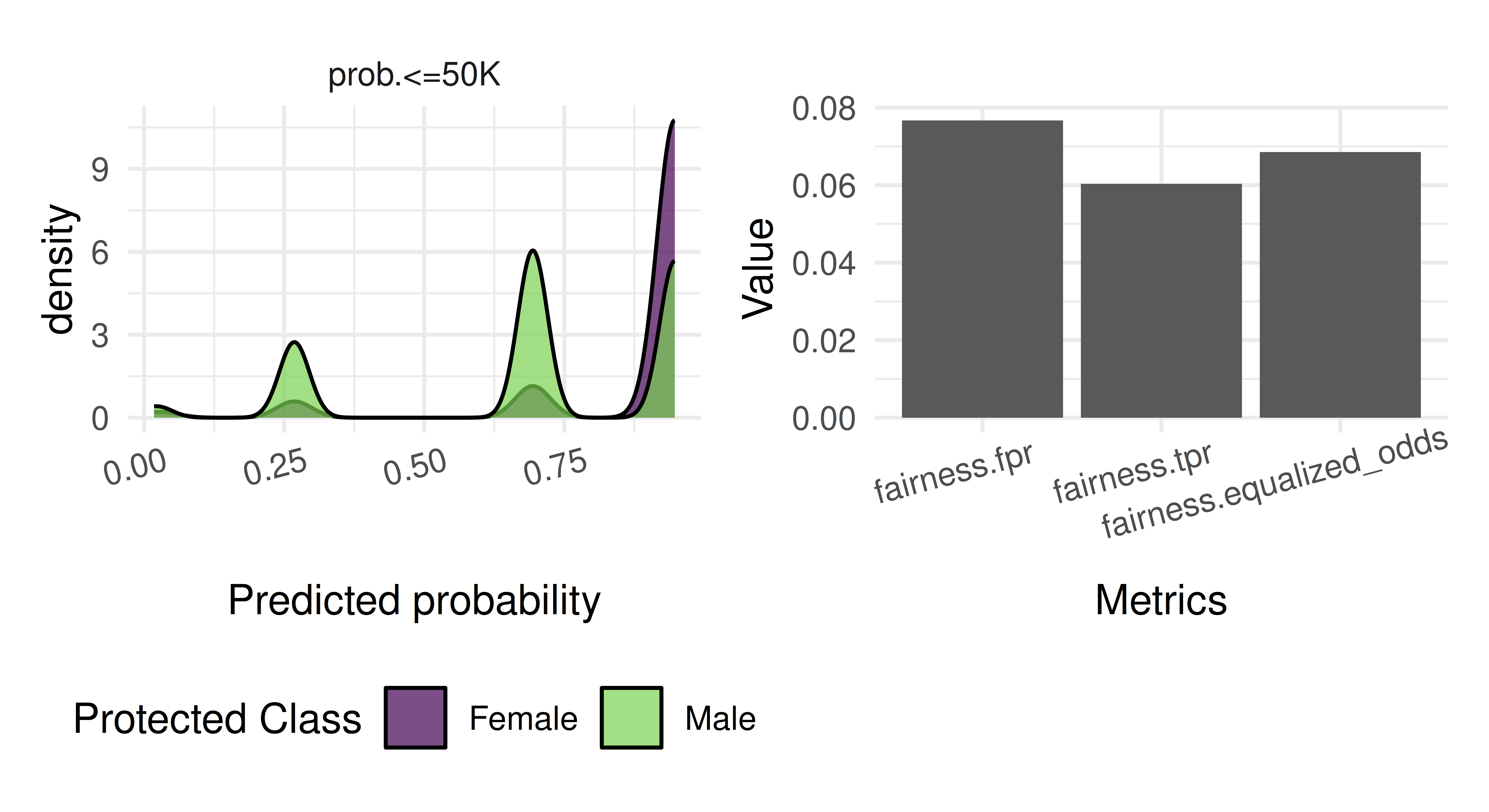
Visualizations can also help better understand discrepancies between groups or differences between models. fairness_prediction_density() plots the sub-group densities across group levels and compare_metrics() scores predictions across multiple metrics:
Figure 14.1: Fairness prediction density plot (left) showing the density of predictions for the positive class split by “Male” and “Female” individuals. The metrics comparison barplot (right) displays the model’s scores across the specified metrics.
In this example (Figure 14.1), we can see the model is more likely to predict ‘Female’ observations as having a lower salary. This could be due to systemic prejudices seen in the data, i.e., women are more likely to have lower salaries due to societal biases, or could be due to bias introduced by the algorithm. As the right plot indicates that all fairness metrics exceed 0.05, this supports the argument that the algorithm may have introduced further bias (with the same caveat about the 0.05 threshold).
14.4 Fair Machine Learning
If we detect that our model is unfair, then a natural next step is to mitigate such biases. mlr3fairness comes with several options to address biases in models, which broadly fall into three categories (Caton and Haas 2020):
Preprocessing data – The underlying data is preprocessed in some way to address bias in the data before it is passed to the Learner;
Employing fair models – Some algorithms can incorporate fairness considerations directly, for example, generalized linear model with fairness constraints (lrn("classif.fairzlrm")).
Postprocessing model predictions – Heuristics/algorithms are applied to the predictions to mitigate biases present in the predictions
All methods often slightly decrease predictive performance and it can therefore be useful to try all approaches to empirically see which balance predictive performance and fairness. In general, all biases should be addressed at their root cause (or as close to it) as possible as any other intervention will be suboptimal.
Pre- and postprocessing schemes can be integrated using mlr3pipelines (Chapter 7). We provide two examples below, first preprocessing to balance observation weights with po("reweighing_wts") and second post-processing predictions using po("EOd"). The latter enforces the equalized odds fairness definition by stochastically flipping specific predictions. We also test lrn("classif.fairzlrm") against the other methods.
Warning
The following code chunks no longer run successfully and have been disabled. The benchmark involving lrn("classif.fairzlrm") currently fails to execute.
# load learnerslrn_rpart=lrn("classif.rpart", predict_type ="prob")lrn_rpart$id="rpart"l1=as_learner(po("reweighing_wts")%>>%lrn("classif.rpart"))l1$id="reweight"l2=as_learner(po("learner_cv", lrn("classif.rpart"))%>>%po("EOd"))l2$id="EOd"# preprocess by collapsing factorsl3=as_learner(po("collapsefactors")%>>%lrn("classif.fairzlrm"))l3$id="fairzlrm"# load task and subset by rows and columnsset.seed(1)task=tsk("adult_train")task$set_col_roles("sex", "pta")$filter(sample(task$nrow, 500))$select(setdiff(task$feature_names, "education_num"))# run experimentlrns=list(lrn_rpart, l1, l2, l3)bmr=benchmark(benchmark_grid(task, lrns, rsmp("cv", folds =5)))meas=msrs(c("classif.acc", "fairness.eod"))bmr$aggregate(meas)[,.(learner_id, classif.acc, fairness.equalized_odds)]
We can study the result using built-in plotting functions, below we use fairness_accuracy_tradeoff(), to compare classification accuracy (default accuracy measure for the function) and equalized odds (msr("fairness.eod")) across cross-validation folds.
Looking at the table of results and ?fig-fairness-tradeoff, the reweighting method appears to yield marginally better fairness metrics than the other methods though the difference is unlikely to be significant. So in this case, we would likely conclude that introducing bias mitigation steps did not improve algorithmic fairness.
As well as manually computing and analyzing fairness metrics, one could also make use of mlr3tuning (Chapter 4) to automate the process with respect to one or more metrics (Section 5.2).
14.5 Conclusion
The functionality introduced above is intended to help users investigate their models for biases and potentially mitigate them. Fairness metrics can not be used to prove or guarantee fairness. Deciding whether a model is fair requires additional investigation, for example, understanding what the measured quantities represent for an individual in the real world and what other biases might exist in the data that could lead to discrepancies in how, for example, covariates or the label are measured.
The simplicity of fairness metrics means they should only be used for exploratory purposes, and practitioners should not solely rely on them to make decisions about employing a machine learning model or assessing whether a system is fair. Instead, practitioners should look beyond the model and consider the data used for training and the process of data and label acquisition. To help in this process, it is important to provide robust documentation for data collection methods, the resulting data, and the models resulting from this data. Informing auditors about those aspects of a deployed model can lead to a better assessment of a model’s fairness. Questionnaires for machine learning models and data sets have been previously proposed in the literature and are available in mlr3fairness from automated report templates (report_modelcard() and report_datasheet()) using R markdown for data sets and machine learning models. In addition, report_fairness() provides a template for a fairness report inspired by the Aequitas Toolkit (Saleiro et al. 2018).
Fairness Report
We hope that pairing the functionality available in mlr3fairness with additional exploratory data analysis, a solid understanding of the societal context in which the decision is made and integrating additional tools (e.g. interpretability methods seen in Chapter 12), might help to mitigate or diminish unfairness in systems deployed in the future.
Table 14.1: Important classes and functions covered in this chapter with underlying class (if applicable), class constructor or function, and important class fields and methods (if applicable).
Train a model of your choice on tsk("adult_train") and test it on tsk("adult_test"), use any measure of your choice to evaluate your predictions. Assume our goal is to achieve parity in false omission rates across the protected ‘sex’ attribute. Construct a fairness metric that encodes this and evaluate your model. To get a deeper understanding, look at the groupwise_metrics function to obtain performance in each group.
Improve your model by employing pipelines that use pre- or post-processing methods for fairness. Evaluate your model along the two metrics and visualize the resulting metrics. Compare the different models using an appropriate visualization.
Add “race” as a second sensitive attribute to your dataset. Add the information to your task and evaluate the initial model again. What changes? Again study the groupwise_metrics.
In this chapter we were unable to reduce bias in our experiment. Using everything you have learned in this book, see if you can successfully reduce bias in your model. Critically reflect on this exercise, why might this be a bad idea?
14.7 Citation
Please cite this chapter as:
Pfisterer F. (2024). Algorithmic Fairness. In Bischl B, Sonabend R, Kotthoff L, Lang M, (Eds.), Applied Machine Learning Using mlr3 in R. CRC Press. https://mlr3book.mlr-org.com/algorithmic_fairness.html.
@incollection{citekey,author = "Florian Pfisterer",title = "Algorithmic Fairness",booktitle = "Applied Machine Learning Using {m}lr3 in {R}",publisher = "CRC Press", year = "2024",editor = "Bernd Bischl and Raphael Sonabend and Lars Kotthoff and Michel Lang",url = "https://mlr3book.mlr-org.com/algorithmic_fairness.html"}
Barocas, Solon, Moritz Hardt, and Arvind Narayanan. 2019. Fairness and Machine Learning: Limitations and Opportunities. fairmlbook.org.
Dua, Dheeru, and Casey Graff. 2017. “UCI Machine Learning Repository.” University of California, Irvine, School of Information; Computer Sciences. https://archive.ics.uci.edu/ml.
Huang, Jonathan, Galal Galal, Mozziyar Etemadi, and Mahesh Vaidyanathan. 2022. “Evaluation and Mitigation of Racial Bias in Clinical Machine Learning Models: Scoping Review.”JMIR Med Inform 10 (5). https://doi.org/10.2196/36388.
Mehrabi, Ninareh, Fred Morstatter, Nripsuta Saxena, Kristina Lerman, and Aram Galstyan. 2021. “A Survey on Bias and Fairness in Machine Learning.”ACM Comput. Surv. 54 (6). https://doi.org/10.1145/3457607.
Mitchell, Shira, Eric Potash, Solon Barocas, Alexander D’Amour, and Kristian Lum. 2021. “Algorithmic Fairness: Choices, Assumptions, and Definitions.”Annual Review of Statistics and Its Application 8: 141–63. https://doi.org/10.1146/annurev-statistics-042720-125902.
Saleiro, Pedro, Benedict Kuester, Abby Stevens, Ari Anisfeld, Loren Hinkson, Jesse London, and Rayid Ghani. 2018. “Aequitas: A Bias and Fairness Audit Toolkit.”arXiv Preprint arXiv:1811.05577. https://doi.org/10.48550/arXiv.1811.05577.
Sonabend, Raphael, Florian Pfisterer, Alan Mishler, Moritz Schauer, Lukas Burk, Sumantrak Mukherjee, and Sebastian Vollmer. 2022. “Flexible Group Fairness Metrics for Survival Analysis.” In DSHealth 2022 Workshop on Applied Data Science for Healthcare at KDD2022. https://arxiv.org/abs/2206.03256.
Wachter, Sandra, Brent Mittelstadt, and Chris Russell. 2021. “Why Fairness Cannot Be Automated: Bridging the Gap Between EU Non-Discrimination Law and AI.”Computer Law & Security Review 41: 105567. https://doi.org/https://doi.org/10.1016/j.clsr.2021.105567.
Source Code
---aliases: - "/algorithmic_fairness.html"---# Algorithmic Fairness {#sec-fairness}{{< include ../../common/_setup.qmd >}}`r chapter = "Algorithmic Fairness"``r authors(chapter)`In this chapter, we will explore `r index('algorithmic fairness')`\index{fairness|see{algorithmic fairness}} in automated decision-making and how we can build fair and unbiased (or at least less biased) predictive models.Methods to help audit and resolve bias in `r mlr3` models are implemented in `r mlr3fairness`.We will begin by first discussing some of the theory behind algorithmic fairness and then show how this is implemented in `mlr3fairness`.Automated decision-making systems based on data-driven models are becoming increasingly common but without proper auditing, these models may result in negative consequences for individuals, especially those from underprivileged groups.The proliferation of such systems in everyday life has made it important to address the potential for biases in these models.As a real-world example, historical and sampling biases have led to better quality medical data for patients from White ethnic groups when compared with other ethnic groups.If a model is trained primarily on data from White patients, then the model may appear 'good' with respect to a given performance metric (e.g., classification error) when in fact the model could simultaneously be making good predictions for White patients while making bad or even harmful predictions for other patients [@Huang2022].As ML-driven systems are used for highly influential decisions, it is vital to develop capabilities to analyze and assess these models not only with respect to their robustness and predictive performance but also with respect to potential biases.As we work through this chapter we will use the `"adult_train"` and `"adult_test"` tasks from `mlr3fairness`, which contain a subset of the `Adult` dataset [@uci].This is a binary classification task to predict if an individual earns more than $50,000 per year and is useful for demonstrating biases in data.```{r algorithmic_fairness-001}library(mlr3fairness)tsk_adult_train =tsk("adult_train")tsk_adult_train```## Bias and FairnessIn the context of fairness, `r index('bias', aside = TRUE)` refers to disparities in how a model treats individuals or groups.In this chapter, we will concentrate on a subset of bias definitions, those concerning `r index('group fairness', aside = TRUE)`.For example, in the adult dataset, it can be seen that adults in the group 'Male' are significantly more likely to earn a salary greater than $50K per year when compared to the group 'Female'.```{r algorithmic_fairness-002}sex_salary =table(tsk_adult_train$data(cols =c("sex", "target")))round(proportions(sex_salary), 2)chisq.test(sex_salary)```In this example, we would refer to the 'sex' variable as a `r index('sensitive attribute', aside = TRUE)`.The goal of group fairness is then to ascertain if decisions are fair across groups defined by a sensitive attribute.The sensitive attribute in a task is set with the `"pta"` (**p**ro**t**ected **a**ttribute) column role (@sec-row-col-roles).```{r algorithmic_fairness-003, eval = FALSE}tsk_adult_train$set_col_roles("sex", add_to ="pta")```If more than one sensitive attribute is specified, then fairness will be based on observations at the intersections of the specified groups.In this chapter we will only focus on group fairness, however, one could also consider auditing individual fairness\index{algorithmic fairness!individual}, which assesses fairness at an individual level, and causal fairness\index{algorithmic fairness!causal}, which incorporates causal relationships in the data and propose metrics based on a directed acyclic graph [@fairmlbook;@mitchell21].While we will only focus on metrics for binary classification here, most metrics discussed naturally extend to more complex scenarios, such as multi-class classification, regression, and survival analysis [@Mehrabi2021; @Sonabend2022a].## Group Fairness NotionsIt is necessary to choose a notion of group fairness before selecting an appropriate fairness metric to measure algorithmic bias.Model predictions are said to be `r index('bias-transforming', aside = TRUE)`[@Wachter2021], or to satisfy independence\index{independence|see{bias-transforming}}, if the predictions made by the model are independent of the sensitive attribute.This group includes the concept of "`r index('Demographic Parity')`", which tests if the proportion of positive predictions (`r index('PPV', "positive predictive value")`) is equal across all groups.Bias-transforming methods (i.e., those that test for independence) do not depend on labels and can help detect biases arising from different base rates across populations.A model is said to be `r index('bias-preserving', aside = TRUE)`, or to satisfy separation\index{separation|see{bias-preserving}}, if the predictions made by the model are independent of the sensitive attribute *given the true label*.In other words, the model should make roughly the same amount of right/wrong predictions in each group.Several metrics fall under this category, such as "`r index('equalized odds')`", which tests if the `r index('TPR', "true positive rate")` and `r index('FPR', "false positive rate")` is equal across groups.Bias-preserving metrics (which test for separation) test if errors made by a model are equal across groups but might not account for bias in the labels (e.g., if outcomes in the real world may be biased such as different rates of arrest for people from different ethnic groups).Choosing a fairness notion will depend on the model's purpose and its societal context.For example, if a model is being used to predict if a person is guilty of something then we might want to focus on false positive or false discovery rates instead of true positives.Whichever metric is chosen, we are essentially condensing systemic biases and prejudices into a few numbers, and all metrics are limited with none being able to identify all biases that may exist in the data.For example, if societal biases lead to disparities in an observed quantity (such as school exam scores) for individuals with the same underlying ability, these metrics may not identify existing biases.To see these notions in practice, let $A$ be a binary sensitive group taking values $0$ and $1$ and let $M$ be a fairness metric.Then to measure independence we would simply calculate the difference between these values and test if the result is less than some threshold, $\epsilon$.$$|\Delta_{M}| = |M_{A=0} - M_{A=1}| < \epsilon$$If we used TPR as our metric $M$ then if $|\Delta_{M}| > \epsilon$ (e.g., $\epsilon = 0.05$) we would conclude that predictions from our model violate the equality of opportunity metric and do not satisfy separation.If we chose accuracy or PPV for $M$, then we would have concluded that the model predictions do not satisfy independence.In `mlr3fairness` we can construct a fairness metric from any `r ref("Measure")` by constructing `msr("fairness", base_measure, range)` with our metric of choice passed to `base_measure` as well as the possible range the metric can take (i.e., the range in differences possible based on the base measure):```{r algorithmic_fairness-004}fair_tpr =msr("fairness", base_measure =msr("classif.tpr"),range =c(0, 1))fair_tpr```We have implemented several `Measure`s in `mlr3fairness` that simplify this step for you, these are named `fairness.<base_measure>`, for example for TPR: `msr("fairness.tpr")` would run the same code as above.## Auditing a Model For BiasWith our sensitive attribute set and the fairness metric selected, we can now train a `r ref("Learner")` and test for bias. Below we use a random forest and evaluate the absolute difference in true positive rate across groups 'Male' and 'Female':```{r algorithmic_fairness-005}tsk_adult_test =tsk("adult_test")lrn_rpart =lrn("classif.rpart", predict_type ="prob")prediction = lrn_rpart$train(tsk_adult_train)$predict(tsk_adult_test)prediction$score(fair_tpr, tsk_adult_test)```With an $\epsilon$ value of $0.05$ we would conclude that there is bias present in our model, however, this value of $\epsilon$ is arbitrary and should be decided based on context.As well as using fairness metrics to evaluate a single model, they can also be used in larger benchmark experiments to compare bias across multiple models.Visualizations can also help better understand discrepancies between groups or differences between models.`r ref("fairness_prediction_density()")` plots the sub-group densities across group levels and `r ref("compare_metrics()")` scores predictions across multiple metrics:```{r algorithmic_fairness-006, message=FALSE, warning=FALSE}#| fig-cap: Fairness prediction density plot (left) showing the density of predictions for the positive class split by "Male" and "Female" individuals. The metrics comparison barplot (right) displays the model's scores across the specified metrics.#| fig-alt: "Two panel plot. Left: Density plot showing that 'Female' observations are more likely to be predicted as having a salary less than $50K than 'Male' observations. Right: Three bar charts for the metrics 'fairness.fpr', 'fairness.tpr', 'fairness.eod' with bars at roughly 0.08, 0.06, and 0.07 respectively."#| label: fig-fairnesslibrary(patchwork)library(ggplot2)p1 =fairness_prediction_density(prediction, task = tsk_adult_test)p2 =compare_metrics(prediction,msrs(c("fairness.fpr", "fairness.tpr", "fairness.eod")),task = tsk_adult_test)(p1 + p2) *theme_minimal() *scale_fill_viridis_d(end =0.8, alpha =0.8) *theme(axis.text.x =element_text(angle =15, hjust = .7),legend.position ="bottom" )```In this example (@fig-fairness), we can see the model is more likely to predict 'Female' observations as having a lower salary.This could be due to systemic prejudices seen in the data, i.e., women are more likely to have lower salaries due to societal biases, or could be due to bias introduced by the algorithm.As the right plot indicates that all fairness metrics exceed 0.05, this supports the argument that the algorithm may have introduced further bias (with the same caveat about the 0.05 threshold).## Fair Machine LearningIf we detect that our model is unfair, then a natural next step is to mitigate such biases.`mlr3fairness` comes with several options to address biases in models, which broadly fall into three categories [@caton-arxiv20a]:1. `r index('Preprocessing')` data -- The underlying data is preprocessed in some way to address bias in the data before it is passed to the `r ref("Learner")`;2. Employing fair models -- Some algorithms can incorporate fairness considerations directly, for example, generalized linear model with fairness constraints (`lrn("classif.fairzlrm")`).3. Postprocessing model predictions -- Heuristics/algorithms are applied to the predictions to mitigate biases present in the predictionsAll methods often slightly decrease predictive performance and it can therefore be useful to try all approaches to empirically see which balance predictive performance and fairness.In general, all biases should be addressed at their root cause (or as close to it) as possible as any other intervention will be suboptimal.Pre- and postprocessing schemes can be integrated using `r mlr3pipelines` (@sec-pipelines).We provide two examples below, first preprocessing to balance observation weights with `po("reweighing_wts")` and second post-processing predictions using `po("EOd")`. The latter enforces the equalized odds fairness definition by stochastically flipping specific predictions.We also test `lrn("classif.fairzlrm")` against the other methods.::: {.callout-warning}The following code chunks no longer run successfully and have been disabled.The benchmark involving `lrn("classif.fairzlrm")` currently fails to execute.:::```{r algorithmic_fairness-007, warning=FALSE, message=FALSE}#| eval: false# load learnerslrn_rpart =lrn("classif.rpart", predict_type ="prob")lrn_rpart$id ="rpart"l1 =as_learner(po("reweighing_wts") %>>%lrn("classif.rpart"))l1$id ="reweight"l2 =as_learner(po("learner_cv", lrn("classif.rpart")) %>>%po("EOd"))l2$id ="EOd"# preprocess by collapsing factorsl3 =as_learner(po("collapsefactors") %>>%lrn("classif.fairzlrm"))l3$id ="fairzlrm"# load task and subset by rows and columnsset.seed(1)task =tsk("adult_train")task$set_col_roles("sex", "pta")$filter(sample(task$nrow, 500))$select(setdiff(task$feature_names, "education_num"))# run experimentlrns =list(lrn_rpart, l1, l2, l3)bmr =benchmark(benchmark_grid(task, lrns, rsmp("cv", folds =5)))meas =msrs(c("classif.acc", "fairness.eod"))bmr$aggregate(meas)[, .(learner_id, classif.acc, fairness.equalized_odds)]```We can study the result using built-in plotting functions, below we use `r ref("fairness_accuracy_tradeoff()")`, to compare classification accuracy (default accuracy measure for the function) and equalized odds (`msr("fairness.eod")`) across cross-validation folds.```{r algorithmic_fairness-008}#| eval: false#| fig-cap: Comparison of learners with respect to classification accuracy (x-axis) and equalized odds (y-axis) across (dots) and aggregated over (crosses) folds.#| fig-alt: "Scatterplot with dots and crosses. x-axis is 'classif.acc' between 0.75 and 0.89, y-axis is 'fairness.equalized_odds' between 0 and 0.4. Plot results described in text."#| label: fig-fairness-tradeofffairness_accuracy_tradeoff(bmr, fairness_measure =msr("fairness.eod"),accuracy_measure =msr("classif.ce")) + ggplot2::scale_color_viridis_d("Learner") + ggplot2::theme_minimal()```Looking at the table of results and @fig-fairness-tradeoff, the reweighting method appears to yield marginally better fairness metrics than the other methods though the difference is unlikely to be significant.So in this case, we would likely conclude that introducing bias mitigation steps did not improve algorithmic fairness.As well as manually computing and analyzing fairness metrics, one could also make use of `r mlr3tuning` (@sec-optimization) to automate the process with respect to one or more metrics (@sec-multi-metrics-tuning).## ConclusionThe functionality introduced above is intended to help users investigate their models for biases and potentially mitigate them.Fairness metrics can not be used to prove or guarantee fairness.Deciding whether a model is fair requires additional investigation, for example, understanding what the measured quantities represent for an individual in the real world and what other biases might exist in the data that could lead to discrepancies in how, for example, covariates or the label are measured.The simplicity of fairness metrics means they should only be used for exploratory purposes, and practitioners should not solely rely on them to make decisions about employing a machine learning model or assessing whether a system is fair.Instead, practitioners should look beyond the model and consider the data used for training and the process of data and label acquisition.To help in this process, it is important to provide robust documentation for data collection methods, the resulting data, and the models resulting from this data.Informing auditors about those aspects of a deployed model can lead to a better assessment of a model's fairness.Questionnaires for machine learning models and data sets have been previously proposed in the literature and are available in `r mlr3fairness` from automated report templates (`r ref("report_modelcard()")` and `r ref("report_datasheet()")`) using R markdown for data sets and machine learning models.In addition, `r ref("report_fairness()")` provides a template for a `r index('fairness report', aside = TRUE)` inspired by the Aequitas Toolkit [@2018aequitas].We hope that pairing the functionality available in `mlr3fairness` with additional exploratory data analysis, a solid understanding of the societal context in which the decision is made and integrating additional tools (e.g. interpretability methods seen in @sec-interpretation), might help to mitigate or diminish unfairness in systems deployed in the future.| Class | Constructor/Function | Fields/Methods || ---| ---| ---||`r ref("MeasureFairness")`|`msr("fairness", ...)`| - || - |`r ref("fairness_prediction_density()")`||| - |`r ref("compare_metrics()")`| - ||`r ref("PipeOpReweighingWeights")`|`po("reweighing_wts")`| - ||`r ref("PipeOpEOd")`|`po("EOd")`| - || - |`r ref("fairness_accuracy_tradeoff()")`||| - |`r ref("report_fairness()")`| - |: Important classes and functions covered in this chapter with underlying class (if applicable), class constructor or function, and important class fields and methods (if applicable). {#tbl-api-fair}## Exercises1. Train a model of your choice on `tsk("adult_train")` and test it on `tsk("adult_test")`, use any measure of your choice to evaluate your predictions. Assume our goal is to achieve parity in false omission rates across the protected 'sex' attribute. Construct a fairness metric that encodes this and evaluate your model. To get a deeper understanding, look at the `r ref("groupwise_metrics")` function to obtain performance in each group.2. Improve your model by employing pipelines that use pre- or post-processing methods for fairness. Evaluate your model along the two metrics and visualize the resulting metrics. Compare the different models using an appropriate visualization.3. Add "race" as a second sensitive attribute to your dataset. Add the information to your task and evaluate the initial model again. What changes? Again study the `groupwise_metrics`.4. In this chapter we were unable to reduce bias in our experiment. Using everything you have learned in this book, see if you can successfully reduce bias in your model. Critically reflect on this exercise, why might this be a bad idea?::: {.content-visible when-format="html"}`r citeas(chapter)`:::