5Advanced Tuning Methods and Black Box Optimization
Lennart Schneider Ludwig-Maximilians-Universität München, and Munich Center for Machine Learning (MCML)
Marc Becker Ludwig-Maximilians-Universität München, and Munich Center for Machine Learning (MCML)
Having looked at the basic usage of mlr3tuning, we will now turn to more advanced methods. We will begin in Section 5.1 by continuing to look at single-objective tuning but will consider what happens when experiments go wrong and how to prevent fatal errors. We will then extend the methodology from Chapter 4 to enable multi-objective tuning, where learners are optimized to multiple measures simultaneously, in Section 5.2 we will demonstrate how this is handled relatively simply in mlr3 by making use of the same classes and methods we have already used. The final two sections focus on specific optimization methods. Section 5.3 looks in detail at multi-fidelity tuning and the Hyperband tuner, and then demonstrates it in practice with mlr3hyperband. Finally, Section 5.4 takes a deep dive into black box Bayesian optimization. This is a more theory-heavy section to motivate the design of the classes and methods in mlr3mbo.
5.1 Error Handling and Memory Management
In this section, we will look at how to use mlr3 to ensure that tuning workflows are efficient and robust. In particular, we will consider how to enable features that prevent fatal errors leading to irrecoverable data loss in the middle of an experiment, and then how to manage tuning experiments that may use up a lot of computer memory.
5.1.1 Encapsulation and Fallback Learner
Error handling is discussed in detail in Section 10.2, however, it is very important in the context of tuning so here we will just practically demonstrate how to make use of encapsulation and fallback learners and explain why they are essential during HPO.
Even in simple machine learning problems, there is a lot of potential for things to go wrong. For example, when learners do not converge, run out of memory, or terminate with an error due to issues in the underlying data. As a common issue, learners can fail if there are factor levels present in the test data that were not in the training data, models fail in this case as there have been no weights/coefficients trained for these new factor levels:
tsk_pen=tsk("penguins")# remove rows with missing valuestsk_pen$filter(tsk_pen$row_ids[complete.cases(tsk_pen$data())])# create custom resampling with new factors in test datarsmp_custom=rsmp("custom")rsmp_custom$instantiate(tsk_pen,list(tsk_pen$row_ids[tsk_pen$data()$island!="Torgersen"]),list(tsk_pen$row_ids[tsk_pen$data()$island=="Torgersen"]))msr_ce=msr("classif.ce")tnr_random=tnr("random_search")learner=lrn("classif.lda", method ="t", nu =to_tune(3, 10))tune(tnr_random, tsk_pen, learner, rsmp_custom, msr_ce, 10)
Error in `lda.default()`:
! variable 6 appears to be constant within groups
In the above example, we can see the tuning process breaks and we lose all information about the hyperparameter optimization process. This is even worse in nested resampling or benchmarking when errors could cause us to lose all progress across multiple configurations or even learners and tasks.
Encapsulation (Section 10.2.1) allows errors to be isolated and handled, without disrupting the tuning process. We can tell a learner to encapsulate an error using the $encapsulate() method as follows:
Note by passing "evaluate", we are telling the learner to set up encapsulation in both the training and prediction stages (see Section 10.2 for other encapsulation options).
Another common issue that cannot be easily solved during HPO is learners not converging and the process running indefinitely. We can prevent this from happening by setting the timeout field in a learner, which signals the learner to stop if it has been running for that much time (in seconds), again this can be set for training and prediction individually:
Now if either an error occurs, or the model timeout threshold is reached, then instead of breaking, the learner will simply not make predictions when errors are found and the result is NA for resampling iterations with errors. When this happens, our hyperparameter optimization experiment will fail as we cannot aggregate results across resampling iterations. Therefore it is essential to select a fallback learner (Section 10.2.2), which is a learner that will be fitted if the learner of interest fails.
A common approach is to use a featureless baseline (lrn("regr.featureless") or lrn("classif.featureless")). We use lrn("classif.featureless"), which always predicts the majority class.
We can now run our experiment and see errors that occurred during tuning in the archive.
# Reading the error in the first resample resultinstance$archive$resample_result(1)$errors
   iteration                                       condition
1:         1 variable 6 appears to be constant within groups
The learner was tuned without breaking because the errors were encapsulated and logged before the fallback learners were used for fitting and predicting:
instance$result
   nu learner_param_vals  x_domain classif.ce
1:  9          <list[2]> <list[1]>          1
5.1.2 Memory Management
Running a large tuning experiment can use a lot of memory, especially when using nested resampling. Most of the memory is consumed by the models since each resampling iteration creates one new model. Storing the models is therefore disabled by default and in most cases is not required. The option store_models in the functions ti() and auto_tuner() allows us to enable the storage of the models.
The archive stores a ResampleResult for each evaluated hyperparameter configuration. The contained Prediction objects can also take up a lot of memory, especially with large datasets and many resampling iterations. We can disable the storage of the resample results by setting store_benchmark_result = FALSE in the functions ti() and auto_tuner(). Note that without the resample results, it is no longer possible to score the configurations with another measure.
The option store_models = TRUE sets store_benchmark_result and store_tuning_instance to TRUE because the models are stored in the benchmark results which in turn is part of the instance. This also means that store_benchmark_result = TRUE sets store_tuning_instance to TRUE.
Finally, we can set store_models = FALSE in the resample() or benchmark() functions to disable the storage of the auto tuners when running nested resampling. This way we can still access the aggregated performance (rr$aggregate()) but lose information about the inner resampling.
5.2 Multi-Objective Tuning
So far we have considered optimizing a model with respect to one metric, but multi-criteria, or multi-objective optimization, is also possible. A simple example of multi-objective optimization might be optimizing a classifier to simultaneously maximize true positive predictions and minimize false negative predictions. In another example, consider the single-objective problem of tuning a neural network to minimize classification error. The best-performing model is likely to be quite complex, possibly with many layers that will have drawbacks like being harder to deploy on devices with limited resources. In this case, we might want to simultaneously minimize the classification error and model complexity.
Multi-objective
By definition, optimization of multiple metrics means these will be in competition (otherwise we would only optimize one of them) and therefore in general no single configuration exists that optimizes all metrics. Therefore, we instead focus on the concept of Pareto optimality. One hyperparameter configuration is said to Pareto-dominate another if the resulting model is equal or better in all metrics and strictly better in at least one metric. For example say we are minimizing classification error, CE, and complexity, CP, for configurations A and B with CE of \(CE_A\) and \(CE_B\) respectively and CP of \(CP_A\) and \(CP_B\) respectively. Then, A pareto-dominates B if: 1) \(CE_A \leq CE_B\) and \(CP_A < CP_B\) or; 2) \(CE_A < CE_B\) and \(CP_A \leq CP_B\). All configurations that are not Pareto-dominated by any other configuration are called Pareto-efficient and the set of all these configurations is the Pareto set. The metric values corresponding to the Pareto set are referred to as the Pareto front.
Pareto front
The goal of multi-objective hyperparameter optimization is to find a set of non-dominated solutions so that their corresponding metric values approximate the Pareto front. We will now demonstrate multi-objective hyperparameter optimization by tuning a decision tree on tsk("sonar") with respect to the classification error, as a measure of model performance, and the number of selected features, as a measure of model complexity (in a decision tree the number of selected features is straightforward to obtain by simply counting the number of unique splitting variables). Methodological details on multi-objective hyperparameter optimization can be found in Karl et al. (2022) and Morales-Hernández, Van Nieuwenhuyse, and Rojas Gonzalez (2022).
As we are tuning with respect to multiple measures, the function ti() automatically creates a TuningInstanceBatchMultiCrit instead of a TuningInstanceBatchSingleCrit. Below we set store_models = TRUE as this is required by the selected features measure.
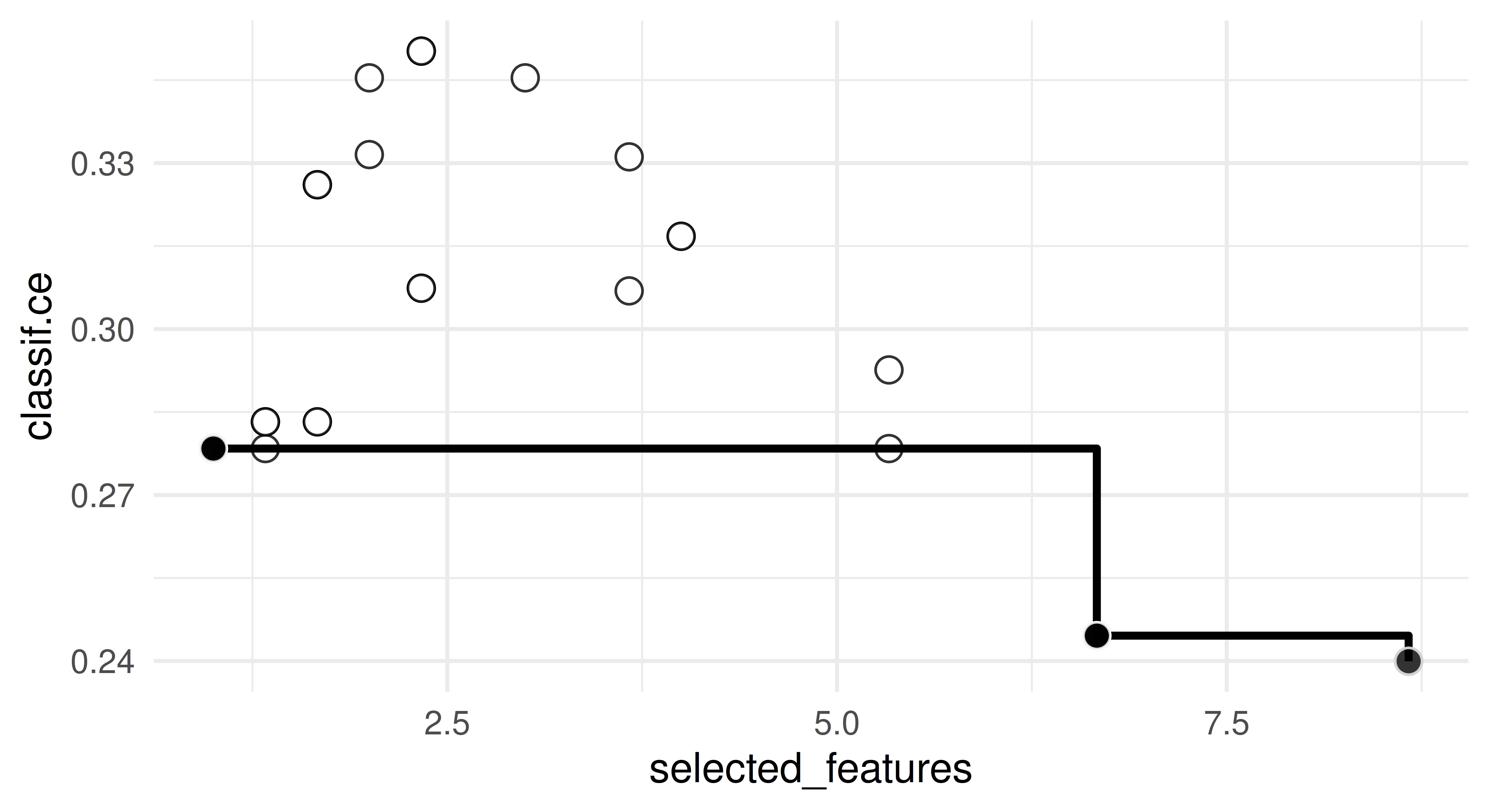
Finally, we inspect the best-performing configurations, i.e., the Pareto set, and visualize the corresponding estimated Pareto front (Figure 5.1). Note that the selected_features measure is averaged across the folds, so the values in the archive may not always be integers.
Figure 5.1: Pareto front of selected features and classification error. White dots represent tested configurations, each black dot individually represents a Pareto-optimal configuration and all black dots together represent the approximated Pareto front.
Determining which configuration to deploy from the Pareto front is up to you. By definition, there is no optimal configuration so this may depend on your use case, for example, if you would prefer lower complexity at the cost of higher error then you might prefer a configuration where selected_features = 1.
You can select one configuration and pass it to a learner for training using $result_learner_param_vals, so if we want to select the second configuration we would run:
As multi-objective tuning requires manual intervention to select a configuration, it is currently not possible to use auto_tuner().
5.3 Multi-Fidelity Tuning via Hyperband
Increasingly large datasets and search spaces and increasingly complex models make hyperparameter optimization a time-consuming and computationally expensive task. To tackle this, some HPO methods make use of evaluating a configuration at multiple fidelity levels. Multi-fidelity HPO is motivated by the idea that the performance of a lower-fidelity model is indicative of the full-fidelity model, which can be used to make HPO more efficient (as we will soon see with Hyperband).
Multi-fidelity HPO
To unpack what these terms mean and to motivate multi-fidelity tuning, say that we think a gradient boosting algorithm with up to 1000 rounds will be a very good fit to our training data. However, we are concerned this model will take too long to tune and train. Therefore, we want to gauge the performance of this model using a similar model that is quicker to train by setting a smaller number of rounds. In this example, the hyperparameter controlling the number of rounds is a fidelity parameter, as it controls the tradeoff between model performance and speed. The different configurations of this parameter are known as fidelity levels. We refer to the model with 1000 rounds as the model at full-fidelity and we want to approximate this model’s performance using models at different fidelity levels. Lower fidelity levels result in low-fidelity models that are quicker to train but may poorly predict the full-fidelity model’s performance. On the other hand, higher fidelity levels result in high-fidelity models that are slower to train but may better indicate the full-fidelity model’s performance.
Other common models that have natural fidelity parameters include neural networks (number of epochs) and random forests (number of trees). The proportion of data to subsample before running any algorithm can also be viewed as a model-agnostic fidelity parameter, we will return to this in Section 8.4.4.
5.3.1 Hyperband and Successive Halving
A popular multi-fidelity HPO algorithm is Hyperband(Li et al. 2018). After having evaluated randomly sampled configurations on low fidelities, Hyperband iteratively allocates more resources to promising configurations and terminates low-performing ones early. Hyperband builds upon the Successive Halving algorithm by Jamieson and Talwalkar (2016). Successive Halving is initialized with a number of starting configurations \(m_0\), the proportion of configurations discarded in each stage \(\eta\), and the minimum, \(r{_{0}}\), and maximum, \(r{_{max}}\), budget (fidelity) of a single evaluation. The algorithm starts by sampling \(m_0\) random configurations and allocating the minimum budget \(r{_{0}}\) to them. The configurations are evaluated and \(\frac{\eta - 1}{\eta}\) of the worst-performing configurations are discarded. The remaining configurations are promoted to the next stage, or ‘bracket’, and evaluated on a larger budget. This continues until one or more configurations are evaluated on the maximum budget \(r{_{max}}\) and the best-performing configuration is selected. The total number of stages is calculated so that each stage consumes approximately the same overall budget. A big disadvantage of this method is that it is unclear if it is better to start with many configurations (large \(m_0\)) and a small budget or fewer configurations (small \(m_0\)) but a larger budget.
Hyperband solves this problem by running Successive Halving with different numbers of starting configurations, each at different budget levels \(r_{0}\). The algorithm is initialized with the same \(\eta\) and \(r_{max}\) parameters (but not \(m_0\)). Each bracket starts with a different budget, \(r_0\), where smaller values mean that more configurations can be evaluated and so the most exploratory bracket (i.e., the one with the most number of stages) is allocated the global minimum budget \(r_{min}\). In each bracket, the starting budget increases by a factor of \(\eta\) until the last bracket essentially performs a random search with the full budget \(r_{max}\). The total number of brackets, \(s_{max} + 1\), is calculated as \(s_{max} = {\log_\eta \frac{r_{max}}{r_{min}}}\). The number of starting configurations \(m_0\) of each bracket are calculated so that each bracket uses approximately the same amount of budget. The optimal hyperparameter configuration in each bracket is the configuration with the best performance in the final stage. The optimal hyperparameter configuration at the end of tuning is the configuration with the best performance across all brackets.
An example Hyperband schedule is given in Table 5.1 where \(s = 3\) is the most exploratory bracket and \(s = 0\) essentially performs a random search using the full budget. Table 5.2 demonstrates how this schedule may look if we were to tune 20 different hyperparameter configurations; note that each entry in the table is a unique ID referring to a possible configuration of multiple hyperparameters to tune.
Table 5.1: Hyperband schedule with the number of configurations, \(m_{i}\), and resources, \(r_{i}\), for each bracket, \(s\), and stage, \(i\), when \(\eta = 2\), \(r{_{min}} = 1\) and \(r{_{max}} = 8\).
\(s = 3\)
\(s = 2\)
\(s = 1\)
\(s = 0\)
\(i\)
\(m_{i}\)
\(r_{i}\)
\(m_{i}\)
\(r_{i}\)
\(m_{i}\)
\(r_{i}\)
\(m_{i}\)
\(r_{i}\)
0
8
1
6
2
4
4
4
8
1
4
2
3
4
2
8
2
2
4
1
8
3
1
8
Table 5.2: Hyperparameter configurations in each stage and bracket from the schedule in Table 5.1. Entries are unique identifiers for tested hyperparameter configurations (HPCs). \(HPC^*_s\) is the optimal hyperparameter configuration in bracket \(s\) and \(HPC^*\) is the optimal hyperparameter configuration across all brackets.
\(s = 3\)
\(s = 2\)
\(s = 1\)
\(s = 0\)
\(i = 0\)
\(\{1, 2, 3, 4, 5, 6, 7, 8\}\)
\(\{9, 10, 11, 12, 13, 14\}\)
\(\{15, 16, 17, 18\}\)
\(\{19, 20, 21, 22\}\)
\(i = 1\)
\(\{1, 2, 7, 8\}\)
\(\{9, 14, 15\}\)
\(\{20, 21\}\)
\(i = 2\)
\(\{1, 8\}\)
\(\{15\}\)
\(i = 3\)
\(\{1\}\)
\(HPC^*_s\)
\(\{1\}\)
\(\{15\}\)
\(\{21\}\)
\(\{22\}\)
\(HPC^*\)
\(\{15\}\)
5.3.2 mlr3hyperband
The Successive Halving and Hyperband algorithms are implemented in mlr3hyperband as tnr("successive_halving") and tnr("hyperband") respectively; in this section, we will only showcase the Hyperband method.
By example, we will optimize lrn("classif.xgboost") on tsk("sonar") and use the number of boosting iterations (nrounds) as the fidelity parameter, this is a suitable choice as increasing iterations increases model training time but generally also improves performance. Hyperband will allocate increasingly more boosting iterations to well-performing hyperparameter configurations.
We will load the learner and define the search space. We specify a range from 16 (\(r_{min}\)) to 128 (\(r_{max}\)) boosting iterations and tag the parameter with "budget" to identify it as a fidelity parameter. For the other hyperparameters, we take the search space for XGBoost from Bischl et al. (2023), which usually works well for a wide range of datasets.
We now construct the tuning instance and a hyperband tuner with eta = 2. We use trm("none") and set the repetitions control parameter to 1 so that Hyperband can terminate itself after all brackets have been evaluated a single time. Note that setting repetition = Inf can be useful if you want a terminator to stop the optimization, for example, based on runtime. The hyperband_schedule() function can be used to display the schedule across the given fidelity levels and budget increase factor.
instance=ti( task =tsk("sonar"), learner =learner, resampling =rsmp("holdout"), measures =msr("classif.ce"), terminator =trm("none"))tuner=tnr("hyperband", eta =2, repetitions =1)hyperband_schedule(r_min =16, r_max =128, eta =2)
Finally, we can tune as normal and print the result and archive. Note that the archive resulting from a Hyperband run contains the additional columns bracket and stage which break down the results by the corresponding bracket and stage.
In this section, we will take a deep dive into Bayesian optimization (BO), also known as Model Based Optimization (MBO). The design of BO is more complex than what we have seen so far in other tuning methods so to help motivate this we will spend a little more time in this section on theory and methodology.
In hyperparameter optimization (Chapter 4), learners are passed a hyperparameter configuration and evaluated on a given task via a resampling technique to estimate its generalization performance with the goal to find the optimal hyperparameter configuration. In general, no analytical description for the mapping from hyperparameter configuration to performance exists and gradient information is also not available. HPO is, therefore, a prime example for black box optimization, which considers the optimization of a function whose mathematical structure and analytical description is unknown or unexploitable. As a result, the only observable information is the output value (i.e., generalization performance) of the function given an input value (i.e., hyperparameter configuration). In fact, as evaluating the performance of a learner can take a substantial amount of time, HPO is quite an expensive black box optimization problem. Black box optimization problems occur in the real-world, for example they are encountered quite often in engineering such as in modeling experiments like crash tests or chemical reactions.
Black Box Optimization
Many optimization algorithm classes exist that can be used for black box optimization, which differ in how they tackle this problem; for example we saw in Chapter 4 methods including grid/random search and briefly discussed evolutionary strategies. Bayesian optimization refers to a class of sample-efficient iterative global black box optimization algorithms that rely on a ‘surrogate model’ trained on observed data to model the black box function. This surrogate model is typically a non-linear regression model that tries to capture the unknown function using limited observed data. During each iteration, BO algorithms employ an ‘acquisition function’ to determine the next candidate point for evaluation. This function measures the expected ‘utility’ of each point within the search space based on the prediction of the surrogate model. The algorithm then selects the candidate point with the best acquisition function value and evaluates the black box function at that point to then update the surrogate model. This iterative process continues until a termination criterion is met, such as reaching a pre-specified maximum number of evaluations or achieving a desired level of performance. BO is a powerful method that often results in good optimization performance, especially if the cost of the black box evaluation becomes expensive and the optimization budget is tight.
In the rest of this section, we will first provide an introduction to black box optimization with the bbotk package and then introduce the building blocks of BO algorithms and examine their interplay and interaction during the optimization process before we assemble these building blocks in a ready to use black box optimizer with mlr3mbo. Readers who are primarily interested in how to utilize BO for HPO without delving deep into the underlying building blocks may want to skip to Section 5.4.4. Detailed introductions to black box optimization and BO are given in Bischl et al. (2023), Feurer and Hutter (2019) and Garnett (2022).
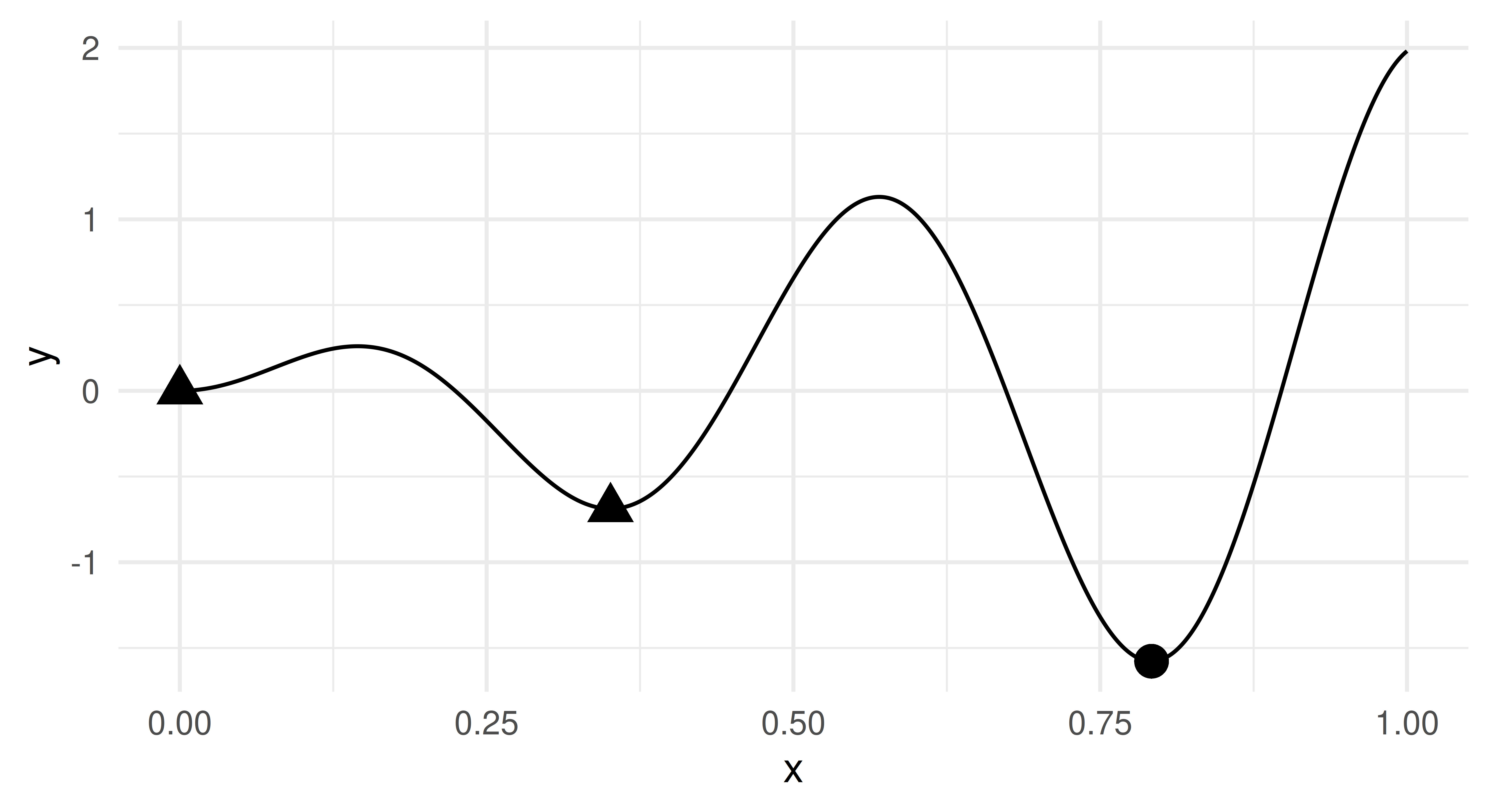
As a running example throughout this section, we will optimize the sinusoidal function \(f: [0, 1] \rightarrow \mathbb{R}, x \mapsto 2x * \sin(14x)\) (Figure 5.2), which is characterized by two local minima and one global minimum.
5.4.1 Black Box Optimization
The bbotk (black box optimization toolkit) package is the workhorse package for general black box optimization within the mlr3 ecosystem. At the heart of the package are the R6 classes:
OptimInstanceBatchSingleCrit relies on an Objective function that wraps the actual mapping from a domain (all possible function inputs) to a codomain (all possible function outputs).
Objective
Objective functions can be created using different classes, all of which inherit from Objective. These classes provide different ways to define and evaluate objective functions and picking the right one will reduce type conversion overhead:
ObjectiveRFun wraps a function that takes a list describing a single configuration as input where elements can be of any type. It is suitable when the underlying function evaluation mechanism is given by evaluating a single configuration at a time.
ObjectiveRFunMany wraps a function that takes a list of multiple configurations as input where elements can be of any type and even mixed types. It is useful when the function evaluation of multiple configurations can be parallelized.
ObjectiveRFunDt wraps a function that operates on a data.table. It allows for efficient vectorized or batched evaluations directly on the data.table object, avoiding unnecessary data type conversions.
To start translating our problem to code we will use the ObjectiveRFun class to take a single configuration as input. The Objective requires specification of the function to optimize its domain and codomain. By tagging the codomain with "minimize" or "maximize" we specify the optimization direction. Note how below our optimization function takes a list as an input with one element called x.
We can visualize our objective by generating a grid of points on which we evaluate the function (Figure 5.2), this will help us identify its local minima and global minimum.
library(ggplot2)xydt=generate_design_grid(domain, resolution =1001)$dataxydt[, y:=objective$eval_dt(xydt)$y]optima=data.table(x =c(0, 0.3509406, 0.7918238))optima[, y:=objective$eval_dt(optima)$y]optima[, type:=c("local", "local", "global")]ggplot(aes(x =x, y =y), data =xydt)+geom_line()+geom_point(aes(pch =type), color ="black", size =4, data =optima)+theme_minimal()+theme(legend.position ="none")
Figure 5.2: Visualization of the sinusoidal function. Local minima in triangles and global minimum in the circle.
The global minimizer, 0.792, corresponds to the point of the domain with the lowest function value:
With the objective function defined, we can proceed to optimize it using OptimInstanceBatchSingleCrit. This class allows us to wrap the objective function and explicitly specify a search space. The search space defines the set of input values we want to optimize over, and it is typically a subset or transformation of the domain, though by default the entire domain is taken as the search space. In black box optimization, it is common for the domain, and hence also the search space, to have finite box constraints. Similarly to HPO, transformations can sometimes be used to more efficiently search the space (Section 4.1.5).
In the following, we use a simple random search to optimize the sinusoidal function over the whole domain and inspect the result from the instance in the usual way (Section 4.1.4). An optimization instance is constructed with the oi() function. Analogously to tuners, Optimizers in bbotk are stored in the mlr_optimizers dictionary and can be constructed with opt().
Similarly to how we can use tune() to construct a tuning instance, here we can use bb_optimize(), which returns a list with elements "par" (best found parameters), "val" (optimal outcome), and "instance" (the optimization instance); the values given as "par" and "val" are the same as the values found in instance$result:
Now we have introduced the basic black box optimization setup, we can introduce the building blocks of any Bayesian optimization algorithm.
5.4.2 Building Blocks of Bayesian Optimization
Bayesian optimization (BO) is a global optimization algorithm that usually follows the following process (Figure 5.3):
Generate and evaluate an initial design
Loop:
Fit a surrogate model on the archive of all observations made so far to model the unknown black box function.
Optimize an acquisition function to determine which points of the search space are promising candidate(s) that should be evaluated next.
Evaluate the next candidate(s) and update the archive of all observations made so far.
Check if a given termination criterion is met, if not go back to (a).
The acquisition function relies on the mean and standard deviation prediction of the surrogate model and requires no evaluation of the true black box function, making it comparably cheap to optimize. A good acquisition function will balance exploiting knowledge about regions where we observed that performance is good and the surrogate model has low uncertainty, with exploring regions where it has not yet evaluated points and as a result the uncertainty of the surrogate model is high.
We refer to these elements as the ‘building blocks’ of BO as it is a highly modular algorithm; as long as the above structure is in place, then the surrogate models, acquisition functions, and acquisition function optimizers are all interchangeable to a certain extent. The design of mlr3mbo reflects this modularity, with the base class for OptimizerMbo holding all the key elements: the BO algorithm loop structure (loop_function), surrogate model (Surrogate), acquisition function (AcqFunction), and acquisition function optimizer (AcqOptimizer). In this section, we will provide a more detailed explanation of these building blocks and explore their interplay and interaction during optimization.
Figure 5.3: Bayesian optimization loop.
5.4.2.1 The Initial Design
Before we can fit a surrogate model to model the unknown black box function, we need data. The initial set of points that is evaluated before a surrogate model can be fit is referred to as the initial design.
mlr3mbo allows you to either construct the initial design manually or let a loop_function construct and evaluate this for you. In this section, we will demonstrate the first method, which requires more user input but therefore allows more control over the initial design.
A simple method to construct an initial design is to use one of the four design generators in paradox:
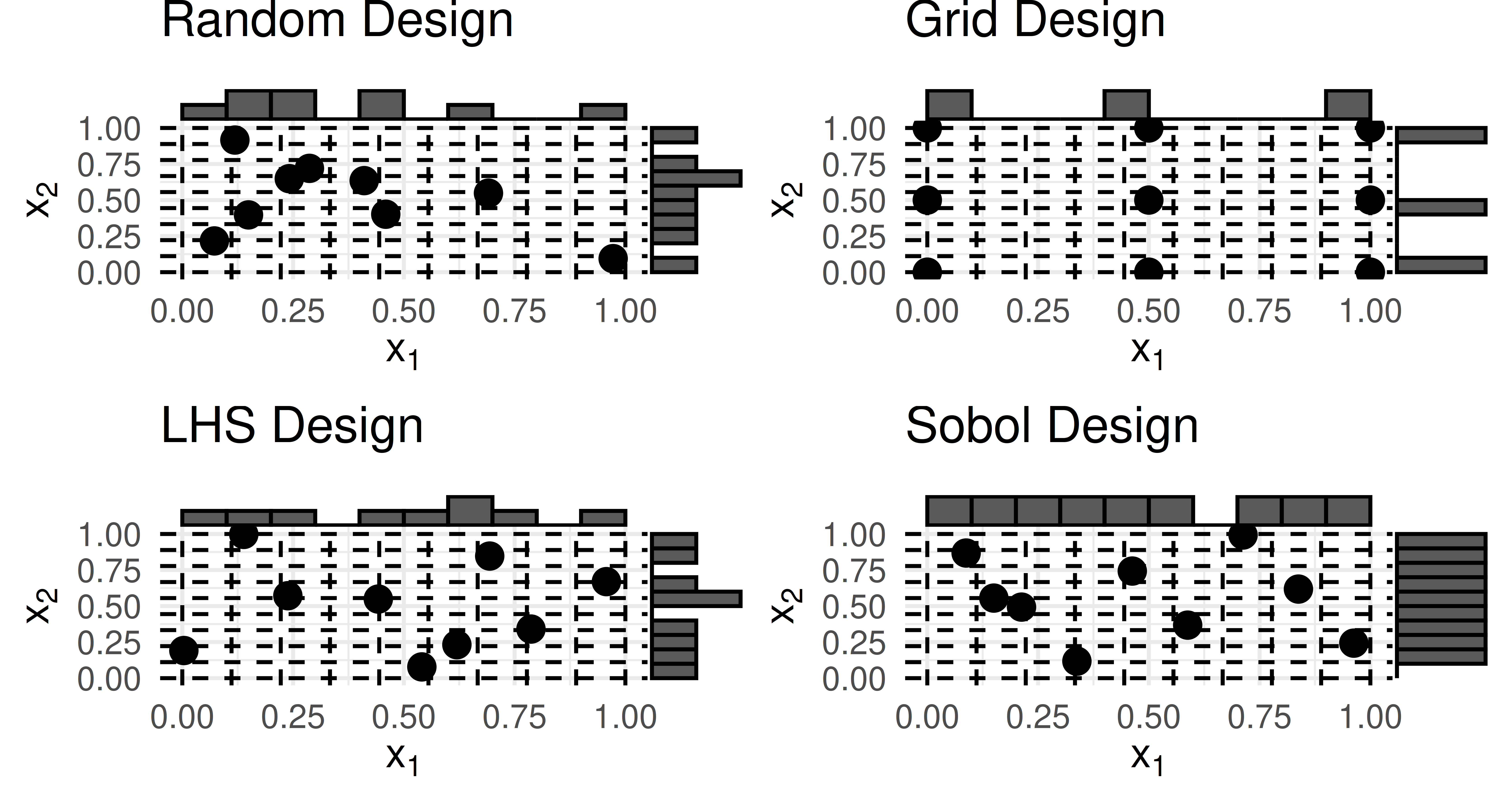
Figure 5.4 illustrates the difference in generated designs from these four methods assuming an initial design of size nine and a domain of two numeric variables from \(0\) to \(1\). We already covered the difference between grid and random designs in Section 4.1.4. An LHS design divides each input variable into equally sized intervals (indicated by the horizontal and vertical dotted lines in Figure 5.4) and ensures that each interval is represented by exactly one sample point, resulting in uniform marginal distributions. Furthermore, in LHS designs the minimal distance between two points is usually maximized, resulting in its space-filling coverage of the space. The Sobol design works similarly to LHS but can provide better coverage than LHS when the number of dimensions is large. For this reason, LHS or Sobol designs are usually recommended for BO, but usually the influence of the initial design will be smaller compared to other design choices of BO. A random design might work well-enough, but grid designs are usually discouraged.
Figure 5.4: Comparing different samplers for constructing an initial design of nine points on a domain of two numeric variables ranging from \(0\) to \(1\). Dotted horizontal and vertical lines partition the domain into equally sized bins. Histograms on the top and right visualize the marginal distributions of the generated sample.
Whichever of these methods you choose, the result is a Design object, which is mostly just a wrapper around a data.table:
Therefore you could also specify a completely custom initial design by defining your own data.table. Either way, when manually constructing an initial design (as opposed to letting loop_function automate this), it needs to be evaluated on the OptimInstance before optimizing it. Returning to our running example of minimizing the sinusoidal function, we will evaluate a custom initial design with $eval_batch():
We can see how each point in our design was evaluated by the sinusoidal function, giving us data we can now use to start the iterative BO algorithm by fitting the surrogate model on that data.
5.4.2.2 Surrogate Model
A surrogate model wraps a regression learner that models the unknown black box function based on observed data. In mlr3mbo, the SurrogateLearner is a higher-level R6 class inheriting from the base Surrogate class, designed to construct and manage the surrogate model, including automatic construction of the TaskRegr that the learner should be trained on at each iteration of the BO loop.
Any regression learner in mlr3 can be used. However, most acquisition functions depend on both mean and standard deviation predictions from the surrogate model, the latter of which requires the "se"predict_type to be supported. Therefore not all learners are suitable for all scenarios. Typical choices of regression learners used as surrogate models include Gaussian processes (lrn("regr.km")) for low to medium dimensional numeric search spaces and random forests (e.g., lrn("regr.ranger")) for higher dimensional mixed (and/or hierarchical) search spaces. A detailed introduction to Gaussian processes can be found in Williams and Rasmussen (2006) and an in-depth focus on Gaussian processes in the context of surrogate models in BO is given in Garnett (2022). In this example, we use a Gaussian process with Matérn 5/2 kernel, which uses BFGS as an optimizer to find the optimal kernel parameters and set trace = FALSE to prevent too much output during fitting.
lrn_gp=lrn("regr.km", covtype ="matern5_2", optim.method ="BFGS", control =list(trace =FALSE))
A SurrogateLearner can be constructed by passing a LearnerRegr object to the sugar function srlrn(), alongside the archive of the instance:
Internally, the regression learner is fit on a TaskRegr where features are the variables of the domain and the target is the codomain, the data is from the Archive of the OptimInstance that is to be optimized.
In our running example we have already initialized our archive with the initial design, so we can update our surrogate model, which essentially fits the Gaussian process, note how we use $learner to access the wrapped model:
Having introduced the concept of a surrogate model, we can now move on to the acquisition function, which makes use of the surrogate model predictions to decide which candidate to evaluate next.
5.4.2.3 Acquisition Function
Roughly speaking, an acquisition function relies on the prediction of a surrogate model and quantifies the expected ‘utility’ of each point of the search space if it were to be evaluated in the next iteration.
A popular example is the expected improvement (Jones, Schonlau, and Welch 1998), which tells us how much we can expect a candidate point to improve over the best function value observed so far (the ‘incumbent’), given the performance prediction of the surrogate model:
Here, \(Y(\mathbf{x)}\) is the surrogate model prediction (a random variable) for a given point \(\mathbf{x}\) (which when using a Gaussian process follows a normal distribution) and \(f_{\mathrm{min}}\) is the best function value observed so far (assuming minimization). Calculating the expected improvement requires mean and standard deviation predictions from the model.
In mlr3mbo, acquisition functions (of class AcqFunction) are stored in the mlr_acqfunctions dictionary and can be constructed with acqf(), passing the key of the method you want to use and our surrogate learner. In our running example, we will use the expected improvement (acqf("ei")) to choose the next candidate for evaluation. Before we can do that, we have to update ($update()) the AcqFunction’s view of the incumbent, to ensure it is still using the best value observed so far.
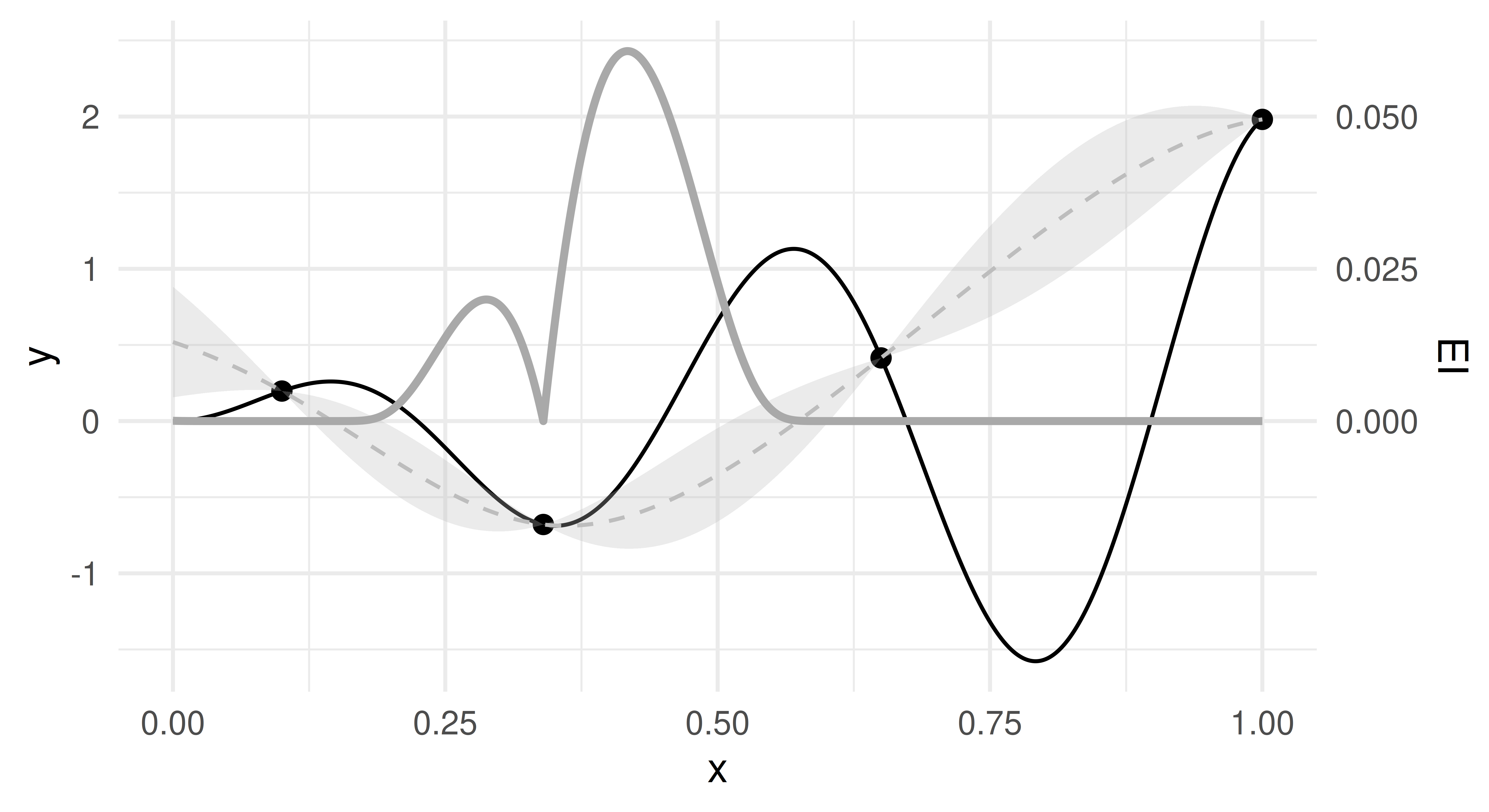
You can use $eval_dt() to evaluate the acquisition function for the domain given as a data.table. In Figure 5.5 we evaluated the expected improvement on a uniform grid of points between \(0\) and \(1\) using the predicted mean and standard deviation from the Gaussian process. We can see that the expected improvement is high in regions where the mean prediction (gray dashed lines) of the Gaussian process is low, or where the uncertainty is high.
Figure 5.5: Expected improvement (solid dark gray line) based on the mean and uncertainty prediction (dashed gray line) of the Gaussian process surrogate model trained on an initial design of four points (black). Ribbons represent the mean plus minus the standard deviation prediction.
We will now proceed to optimize the acquisition function itself to find the candidate with the largest expected improvement.
5.4.2.4 Acquisition Function Optimizer
An acquisition function optimizer of class AcqOptimizer is used to optimize the acquisition function by efficiently searching the space of potential candidates within a limited computational budget.
AcqOptimizer
Due to the non-convex nature of most commonly used acquisition functions (Garnett 2022) it is typical to employ global optimization techniques for acquisition function optimization. Widely used approaches for optimizing acquisition functions include derivative-free global optimization methods like branch and bound algorithms, such as the DIRECT algorithm (Jones, Perttunen, and Stuckman 1993), as well as multi-start local optimization methods, such as running the L-BFGS-B algorithm (Byrd et al. 1995) or a local search multiple times from various starting points (Kim and Choi 2021). Consequently the optimization problem of the acquisition function can be handled as a black box optimization problem itself, but a much cheaper one than the original.
AcqOptimizer objects are constructed with acqo(), which takes as input a Optimizer, a Terminator, and the acquisition function. Optimizers are stored in the mlr_optimizers dictionary and can be constructed with the sugar function opt(). The terminators are the same as those introduced in Section 4.1.2.
Below we use the DIRECT algorithm and we terminate the acquisition function optimization if there is no improvement of at least 1e-5 for 100 iterations. The $optimize() method optimizes the acquisition function and returns the next candidate.
        x  acq_ei  x_domain .already_evaluated
1: 0.4173 0.06074 <list[1]>              FALSE
We have now shown how to run a single iteration of the BO algorithm loop manually. In practice, one would use OptimizerMbo to put all these pieces together to automate the process. Before demonstrating this class we will first take a step back and introduce the loop_function which tells the algorithm how it should be run.
5.4.2.5 Using and Building Loop Functions
The loop_function determines the behavior of the BO algorithm on a global level, i.e., how to define the subroutine that is performed at each iteration to generate new candidates for evaluation. Loop functions are relatively simple functions that take as input the classes that we have just discussed and define the BO loop. Loop functions are stored in the mlr_loop_functions dictionary. As these are S3 (not R6) classes, they can be simply loaded by just referencing the key (i.e., there is no constructor required).
You could pick and use one of the loop functions included in the dictionary above, or you can write your own for finer control over the BO process. A common choice of loop function is the Efficient Global Optimization (EGO) algorithm (Jones, Schonlau, and Welch 1998) (bayesopt_ego()). A simplified version of this code is shown at the end of this section, both to help demonstrate the EGO algorithm, and to give an example of how to write a custom BO variant yourself. In short, the code sets up the relevant components discussed above and then loops the steps above: 1) update the surrogate model 2) update the acquisition function 3) optimize the acquisition function to yield a new candidate 4) evaluate the candidate and add it to the archive. If there is an error during the loop then a fallback is used where the next candidate is proposed uniformly at random, ensuring that the process continues even in the presence of potential issues, we will return to this in Section 5.4.6.
my_simple_ego=function(instance,surrogate,acq_function,acq_optimizer,init_design_size){# setting up the building blockssurrogate$archive=instance$archive# archiveacq_function$surrogate=surrogate# surrogate modelacq_optimizer$acq_function=acq_function# acquisition functionsearch_space=instance$search_space# initial designdesign=generate_design_sobol(search_space, n =init_design_size)$datainstance$eval_batch(design)# MBO looprepeat{candidate=tryCatch({# update the surrogate modelacq_function$surrogate$update()# update the acquisition functionacq_function$update()# optimize the acquisition function to yield a new candidateacq_optimizer$optimize()}, mbo_error =function(mbo_error_condition){generate_design_random(search_space, n =1L)$data})# evaluate the candidate and add it to the archivetryCatch({instance$eval_batch(candidate)}, terminated_error =function(cond){# $eval_batch() throws a terminated_error if the instance is# already terminated, e.g. because of timeout.})if(instance$is_terminated)break}return(instance)}
We are now ready to put everything together to automate the BO process.
5.4.3 Automating BO with OptimizerMbo
OptimizerMbo can be used to assemble the building blocks described above into a single object that can then be used for optimization. We use the bayesopt_ego loop function provided by mlr_loop_functions, which works similarly to the code shown above but takes more care to offer sensible default values for its arguments and handle edge cases correctly. You do not need to pass any of these building blocks to each other manually as the opt() constructor will do this for you:
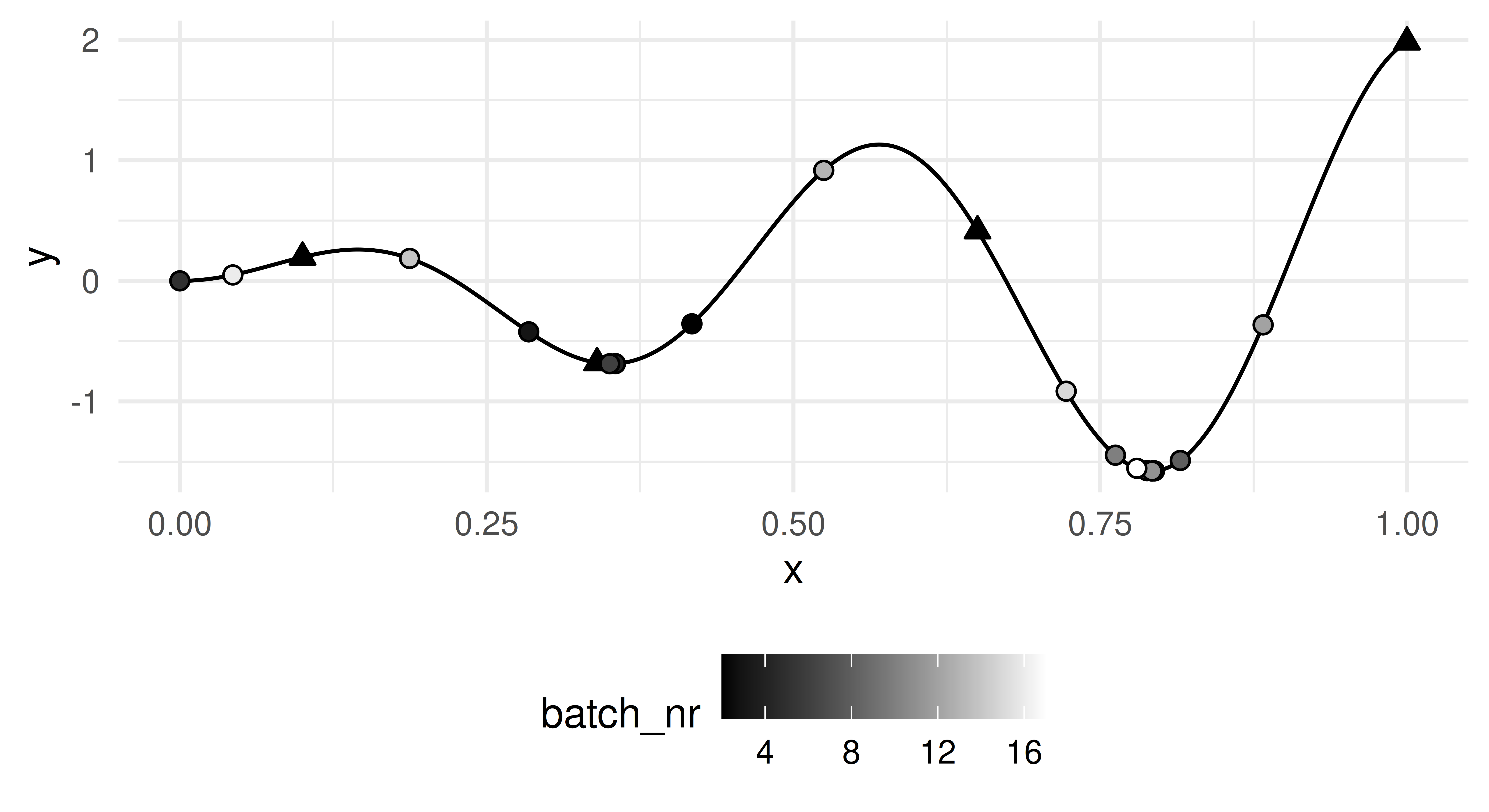
Using only a few evaluations, BO comes close to the true global optimum (0.792). Figure 5.6 shows the sampling trajectory of candidates as the algorithm progressed, we can see that focus is increasingly given to more regions around the global optimum. However, even in later optimization stages, the algorithm still explores new areas, illustrating that the expected improvement acquisition function indeed balances exploration and exploitation as we required.
Figure 5.6: Sampling trajectory of the BO algorithm. Points of the initial design in black triangles. Sampled points are in dots with color progressing from black to white as the algorithm progresses.
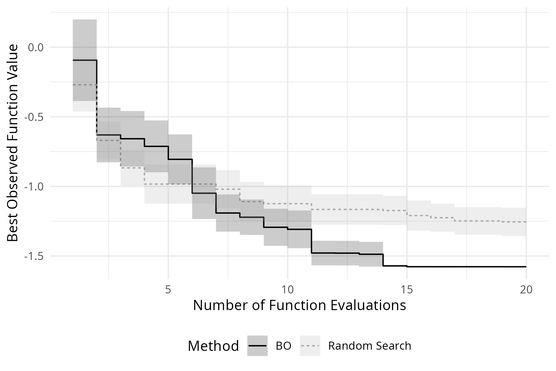
If we replicate running our BO algorithm ten times (with random initial designs and varying random seeds) and compare this to a random search, we can see that BO indeed performs much better and on average reaches the global optimum after around 15 function evaluations (Figure 5.7). As expected, the performance for the initial design size is close to the performance of the random search.
Figure 5.7: Anytime performance of BO and random search on the 1D sinusoidal function given a budget of 20 function evaluations. Solid line depicts the best observed target value averaged over 10 replications. Ribbons represent standard errors.
5.4.4 Bayesian Optimization for HPO
mlr3mbo can be used for HPO by making use of TunerMbo, which is a wrapper around OptimizerMbo and works in the exact same way. As an example, below we will tune the cost and gamma parameters of lrn("classif.svm") with a radial kernel on tsk("sonar") with three-fold CV. We set up tnr("mbo") using the same objects constructed above and then run our tuning experiment as usual:
Multi-objective tuning is also possible with BO with algorithms using many different design choices, for example, whether they use a scalarization approach of objectives and only rely on a single surrogate model, or fit a surrogate model for each objective. More details on multi-objective BO can for example be found in Horn et al. (2015) or Morales-Hernández, Van Nieuwenhuyse, and Rojas Gonzalez (2022).
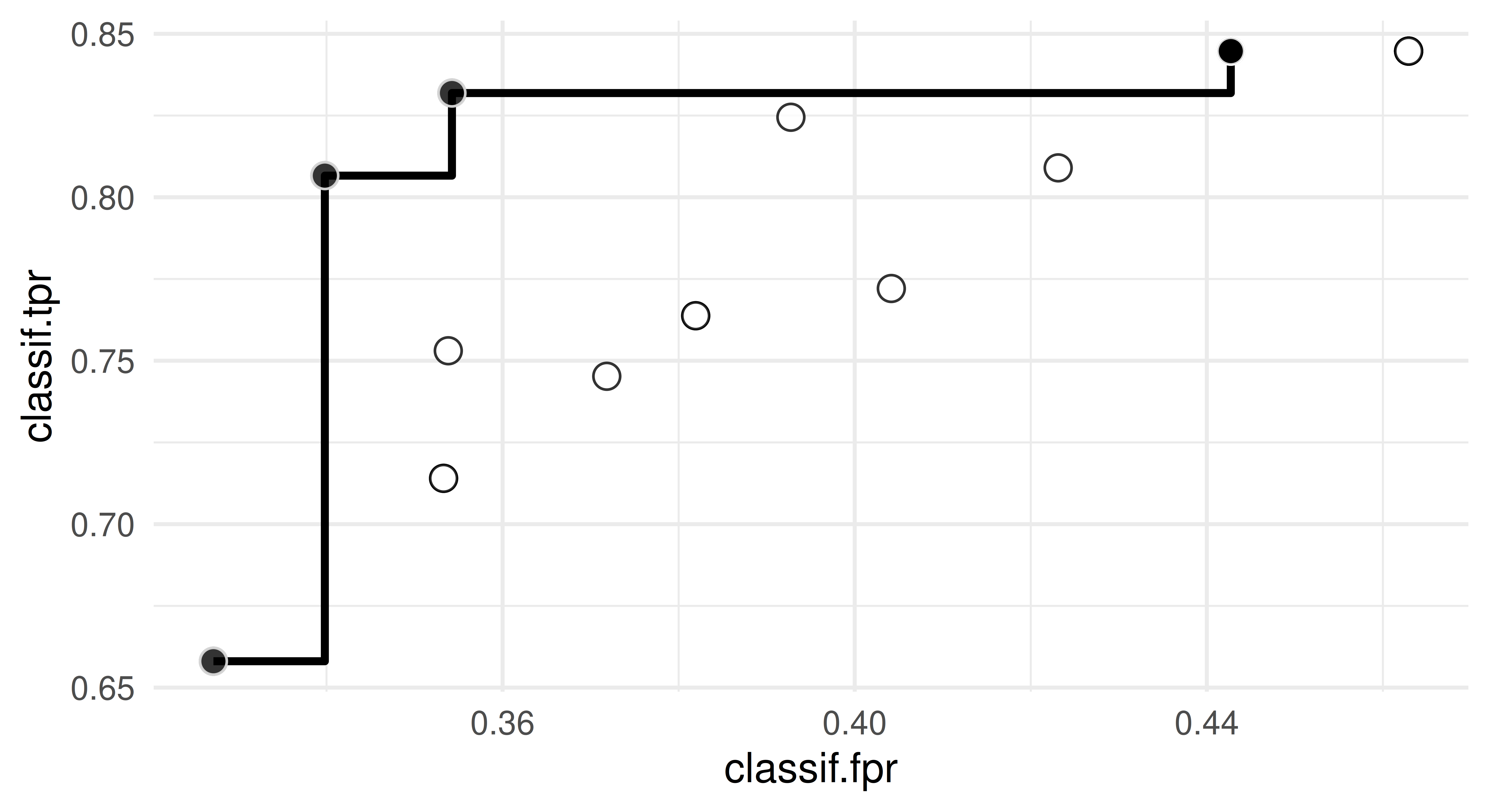
Below we will illustrate multi-objective tuning using the ParEGO (Knowles 2006) loop function. ParEGO (bayesopt_parego()) tackles multi-objective BO via a randomized scalarization approach and models a single scalarized objective function via a single surrogate model and then proceeds to find the next candidate for evaluation making use of a standard single-objective acquisition function such as the expected improvement. Other compatible loop functions can be found by looking at the "instance" column of mlr_loop_functions. We will tune three parameters of a decision tree with respect to the true positive (maximize) and false positive (minimize) rates, the Pareto front is visualized in Figure 5.8.
Figure 5.8: Pareto front of TPR and FPR obtained via ParEGO. White dots represent tested configurations, each black dot individually represents a Pareto-optimal configuration and all black dots together represent the Pareto front.
5.4.5 Noisy Bayesian Optimization
So far, we implicitly assumed that the black box function we are trying to optimize is deterministic, i.e., repeatedly evaluating the same point will always return the same objective function value. However, real-world black box functions are often noisy, which means that repeatedly evaluating the same point will return different objective function values due to background noise on top of the black box function. For example, if you were modeling a machine in a factory to estimate the rate of production, even if all parameters of the machine were controlled, we would still expect different performance at different times due to uncontrollable background factors such as environmental conditions.
In bbotk, you can mark an Objective object as noisy by passing the "noisy" tag to the properties parameter, which allows us to use methods that can treat such objectives differently.
Noisy objectives can be treated in different ways:
A surrogate model can be used to incorporate the noise
An acquisition function can be used that respects noisiness
The final best point(s) after optimization (i.e., the $result field of the instance) can be chosen in a way to reflect noisiness
In the first case, instead of using an interpolating Gaussian process, we could instead use Gaussian process regression that estimates the measurement error by setting nugget.estim = TRUE:
This will result in the Gaussian process not perfectly interpolating training data and the standard deviation prediction associated with the training data will be non-zero, reflecting the uncertainty in the observed function values due to the measurement error. A more in-depth discussion of noise-free vs. noisy observations in the context of Gaussian processes can be found in Chapter 2 of Williams and Rasmussen (2006).
For the second option, one example of an acquisition function that respects noisiness is the Augmented expected improvement (Huang et al. 2012) (acqf("aei")) which essentially rescales the expected improvement, taking measurement error into account.
Finally, mlr3mbo allows for explicitly specifying how the final result after optimization is assigned to the instance (i.e., what will be saved in instance$result) with a result assigner, which can be specified during the construction of an OptimizerMbo or TunerMbo. ResultAssignerSurrogate uses a surrogate model to predict the mean of all evaluated points and proceeds to choose the point with the best mean prediction as the final optimization result. In contrast, the default method, ResultAssignerArchive, just picks the best point according to the evaluations logged in archive. Result assigners are stored in the mlr_result_assigners dictionary and can be constructed with ras().
5.4.6 Practical Considerations in Bayesian Optimization
mlr3mbo tries to use reasonable defaults regarding the choice of surrogate model, acquisition function, acquisition function optimizer and even the loop function. For example, in the case of a purely numeric search space, mlr3mbo will by default use a Gaussian process as the surrogate model and a random forest as the fallback learner and additionally encapsulates the learner (Section 5.1.1). In the case of a mixed or hierarchical search space, mlr3mbo will use a random forest as the surrogate model. Therefore, users can perform BO without specifying any deviation from the defaults and still expect decent optimization performance. To see an up-to-date overview of these defaults, take a look at the help page of mbo_defaults. We will finish this section with some practical considerations to think about when using BO.
Error Handling
In the context of BO, there is plenty of room for potential failure of building blocks which could break the whole process. For example, if two points in the training data are too close to each other, fitting the Gaussian process surrogate model can fail.
mlr3mbo has several built-in safety nets to catch errors. Surrogate includes the catch_errors configuration control parameter, which, if set to TRUE, catches all errors that occur during training or updating of the surrogate model. AcqOptimizer also has the catch_errors configuration control parameter, which can be used to catch all errors that occur during the acquisition function optimization, either due to the surrogate model failing to predict or the acquisition function optimizer erroring. If errors are caught in any of these steps, the standard behavior of any loop_function is to trigger a fallback, which proposes the next candidate uniformly at random. Note, when setting catch_errors = TRUE for the AcqOptimizer, it is usually not necessary to also explicitly set catch_errors = TRUE for the Surrogate, though this may be useful when debugging.
In the worst-case scenario, if all iterations errored, the BO algorithm will simply perform a random search. Ideally, fallback learners (Section 5.1.1) should also be used, which will be employed before proposing the next candidate randomly. The value of the acquisition function is also always logged in the archive of the optimization instance so inspecting this is a good idea to ensure the algorithm behaved as expected.
Surrogate Models
In practice, users may prefer a more robust BO variant over a potentially better-performing but unstable variant. Even if the catch_errors parameters are turned on and are never triggered, that does not guarantee that the BO algorithm ran as intended. For instance, Gaussian processes are sensitive to the choice of kernel and kernel parameters, typically estimated through maximum likelihood estimation, suboptimal parameter values can result in white noise models with a constant mean and standard deviation prediction. In this case, the surrogate model will not provide useful mean and standard deviation predictions resulting in poor overall performance of the BO algorithm. Another practical consideration regarding the choice of surrogate model can be overhead. Fitting a vanilla Gaussian process scales cubically in the number of data points and therefore the overhead of the BO algorithm grows with the number of iterations. Furthermore, vanilla Gaussian processes natively cannot handle categorical input variables or dependencies in the search space (recall that in HPO we often deal with mixed hierarchical spaces). In contrast, a random forest – popularly used as a surrogate model in SMAC(Lindauer et al. 2022) – is cheap to train, quite robust in the sense that it is not as sensitive to its hyperparameters as a Gaussian process, and can easily handle mixed hierarchical spaces. On the downside, a random forest is not really Bayesian (i.e., there is no posterior predictive distribution) and suffers from poor uncertainty estimates and poor extrapolation.
Warmstarting
Warmstarting is a technique in optimization where previous optimization runs are used to improve the convergence rate and final solution of a new, related optimization run. In BO, warmstarting can be achieved by providing a set of likely well-performing configurations as part of the initial design (see, e.g., Feurer, Springenberg, and Hutter 2015). This approach can be particularly advantageous because it allows the surrogate model to start with prior knowledge of the optimization landscape in relevant regions. In mlr3mbo, warmstarting is straightforward by specifying a custom initial design. Furthermore, a convenient feature of mlr3mbo is the ability to continue optimization in an online fashion even after an optimization run has been terminated. Both OptimizerMbo and TunerMbo support this feature, allowing optimization to resume on a given instance even if the optimization was previously interrupted or terminated.
Termination
Common termination criteria include stopping after a fixed number of evaluations, once a given walltime budget has been reached, when performance reaches a certain level, or when performance improvement stagnates. In the context of BO, it can also be sensible to stop the optimization if the best acquisition function value falls below a certain threshold. For instance, terminating the optimization if the expected improvement of the next candidate(s) is negligible can be a reasonable approach. At the time of publishing, terminators based on acquisition functions have not been implemented but this feature will be coming soon.
Parallelization
The standard behavior of most BO algorithms is to sequentially propose a single candidate that should be evaluated next. Users may want to use parallelization to compute candidates more efficiently. If you are using BO for HPO, then the most efficient method is to parallelize the nested resampling, see Section 10.1.4. Alternatively, if the loop function supports candidates being proposed in batches (e.g., bayesopt_parego()) then the q argument to the loop function can be set to propose q candidates in each iteration that can be evaluated in parallel if the Objective is properly implemented.
5.5 Conclusion
In this chapter, we looked at advanced tuning methods. We started by thinking about the types of errors that can occur during tuning and how to handle these to ensure your HPO process does not crash. We presented multi-objective tuning, which can be used to optimize performance measures simultaneously. We then looked at multi-fidelity tuning, in which the Hyberband tuner can be used to efficiently tune algorithms by making use of lower-fidelity evaluations to approximate full-fidelity model performance. We will return to Hyperband in Section 8.4.4 where we will learn how to make use of pipelines in order to tune any algorithm with Hyperband. Finally, we took a deep dive into Bayesian optimization to look at how bbotk, mlr3mbo, and mlr3tuning can be used together to implement complex BO tuning algorithms in mlr3, allowing for highly flexible and sample-efficient algorithms. In the next chapter we will look at feature selection and see how mlr3filters and mlr3fselect use a very similar design interface to mlr3tuning.
Table 5.3: Important classes and functions covered in this chapter with underlying class (if applicable), class constructor or function, and important class methods (if applicable).
Tune the mtry, sample.fraction, and num.trees hyperparameters of lrn("regr.ranger") on tsk("mtcars") and evaluate this with a three-fold CV and the root mean squared error (same as Chapter 4, Exercise 1). Use tnr("mbo") with 50 evaluations. Compare this with the performance progress of a random search run from Chapter 4, Exercise 1. Plot the progress of performance over iterations and visualize the spatial distribution of the evaluated hyperparameter configurations for both algorithms.
Minimize the 2D Rastrigin function \(f: [-5.12, 5.12] \times [-5.12, 5.12] \rightarrow \mathbb{R}\), \(\mathbf{x} \mapsto 10 D+\sum_{i=1}^D\left[x_i^2-10 \cos \left(2 \pi x_i\right)\right]\), \(D = 2\) via BO (standard sequential single-objective BO via bayesopt_ego()) using the lower confidence bound with lambda = 1 as acquisition function and "NLOPT_GN_ORIG_DIRECT" via opt("nloptr") as acquisition function optimizer. Use a budget of 40 function evaluations. Run this with both the “default” Gaussian process surrogate model with Matérn 5/2 kernel, and the “default” random forest surrogate model. Compare their anytime performance (similarly as in Figure 5.7). You can construct the surrogate models with default settings using:
Minimize the following function: \(f: [-10, 10] \rightarrow \mathbb{R}^2, x \mapsto \left(x^2, (x - 2)^2\right)\) with respect to both objectives. Use the ParEGO algorithm. Construct the objective function using the ObjectiveRFunMany class. Terminate the optimization after a runtime of 100 evals. Plot the resulting Pareto front and compare it to the analytical solution, \(y_2 = \left(\sqrt{y_1}-2\right)^2\) with \(y_1\) ranging from \(0\) to \(4\).
5.7 Citation
Please cite this chapter as:
Schneider L, Becker M. (2024). Advanced Tuning Methods and Black Box Optimization. In Bischl B, Sonabend R, Kotthoff L, Lang M, (Eds.), Applied Machine Learning Using mlr3 in R. CRC Press. https://mlr3book.mlr-org.com/advanced_tuning_methods_and_black_box_optimization.html.
@incollection{citekey,author = "Lennart Schneider and Marc Becker",title = "Advanced Tuning Methods and Black Box Optimization",booktitle = "Applied Machine Learning Using {m}lr3 in {R}",publisher = "CRC Press", year = "2024",editor = "Bernd Bischl and Raphael Sonabend and Lars Kotthoff and Michel Lang",url = "https://mlr3book.mlr-org.com/advanced_tuning_methods_and_black_box_optimization.html"}
Bischl, Bernd, Martin Binder, Michel Lang, Tobias Pielok, Jakob Richter, Stefan Coors, Janek Thomas, et al. 2023. “Hyperparameter Optimization: Foundations, Algorithms, Best Practices, and Open Challenges.”Wiley Interdisciplinary Reviews: Data Mining and Knowledge Discovery, e1484. https://doi.org/10.1002/widm.1484.
Byrd, Richard H., Peihuang Lu, Jorge Nocedal, and Ciyou Zhu. 1995. “A Limited Memory Algorithm for Bound Constrained Optimization.”SIAM Journal on Scientific Computing 16 (5): 1190–1208. https://doi.org/10.1137/0916069.
Feurer, Matthias, and Frank Hutter. 2019. “Hyperparameter Optimization.” In Automated Machine Learning: Methods, Systems, Challenges, edited by Frank Hutter, Lars Kotthoff, and Joaquin Vanschoren, 3–33. Cham: Springer International Publishing. https://doi.org/10.1007/978-3-030-05318-5_1.
Feurer, Matthias, Jost Springenberg, and Frank Hutter. 2015. “Initializing Bayesian Hyperparameter Optimization via Meta-Learning.” In Proceedings of the AAAI Conference on Artificial Intelligence. Vol. 29. 1. https://doi.org/10.1609/aaai.v29i1.9354.
Horn, Daniel, Tobias Wagner, Dirk Biermann, Claus Weihs, and Bernd Bischl. 2015. “Model-Based Multi-Objective Optimization: Taxonomy, Multi-Point Proposal, Toolbox and Benchmark.” In Evolutionary Multi-Criterion Optimization, edited by António Gaspar-Cunha, Carlos Henggeler Antunes, and Carlos Coello Coello, 64–78. https://doi.org/10.1007/978-3-319-15934-8_5.
Huang, D., T. T. Allen, W. I. Notz, and N. Zheng. 2012. “Erratum to: Global Optimization of Stochastic Black-Box Systems via Sequential Kriging Meta-Models.”Journal of Global Optimization 54 (2): 431–31. https://doi.org/10.1007/s10898-011-9821-z.
Jamieson, Kevin, and Ameet Talwalkar. 2016. “Non-Stochastic Best Arm Identification and Hyperparameter Optimization.” In Proceedings of the 19th International Conference on Artificial Intelligence and Statistics, edited by Arthur Gretton and Christian C. Robert, 51:240–48. Proceedings of Machine Learning Research. Cadiz, Spain: PMLR. https://proceedings.mlr.press/v51/jamieson16.html.
Jones, Donald R., Cary D. Perttunen, and Bruce E. Stuckman. 1993. “Lipschitzian Optimization Without the Lipschitz Constant.”Journal of Optimization Theory and Applications 79 (1): 157–81. https://doi.org/10.1007/BF00941892.
Jones, Donald R., Matthias Schonlau, and William J. Welch. 1998. “Efficient Global Optimization of Expensive Black-Box Functions.”Journal of Global Optimization 13 (4): 455–92. https://doi.org/10.1023/A:1008306431147.
Karl, Florian, Tobias Pielok, Julia Moosbauer, Florian Pfisterer, Stefan Coors, Martin Binder, Lennart Schneider, et al. 2022. “Multi-Objective Hyperparameter Optimization–an Overview.”arXiv Preprint arXiv:2206.07438. https://doi.org/10.48550/arXiv.2206.07438.
Kim, Jungtaek, and Seungjin Choi. 2021. “On Local Optimizers of Acquisition Functions in Bayesian Optimization.” In Machine Learning and Knowledge Discovery in Databases, edited by Frank Hutter, Kristian Kersting, Jefrey Lijffijt, and Isabel Valera, 675–90. https://doi.org/10.1007/978-3-030-67661-2_40.
Knowles, Joshua. 2006. “ParEGO: A Hybrid Algorithm with on-Line Landscape Approximation for Expensive Multiobjective Optimization Problems.”IEEE Transactions on Evolutionary Computation 10 (1): 50–66. https://doi.org/10.1109/TEVC.2005.851274.
Li, Lisha, Kevin Jamieson, Giulia DeSalvo, Afshin Rostamizadeh, and Ameet Talwalkar. 2018. “Hyperband: A Novel Bandit-Based Approach to Hyperparameter Optimization.”Journal of Machine Learning Research 18 (185): 1–52. https://jmlr.org/papers/v18/16-558.html.
Lindauer, Marius, Katharina Eggensperger, Matthias Feurer, André Biedenkapp, Difan Deng, Carolin Benjamins, Tim Ruhkopf, René Sass, and Frank Hutter. 2022. “SMAC3: A Versatile Bayesian Optimization Package for Hyperparameter Optimization.”Journal of Machine Learning Research 23 (54): 1–9. https://www.jmlr.org/papers/v23/21-0888.html.
Morales-Hernández, Alejandro, Inneke Van Nieuwenhuyse, and Sebastian Rojas Gonzalez. 2022. “A Survey on Multi-Objective Hyperparameter Optimization Algorithms for Machine Learning.”Artificial Intelligence Review, 1–51. https://doi.org/10.1007/s10462-022-10359-2.
Stein, Michael. 1987. “Large Sample Properties of Simulations Using Latin Hypercube Sampling.”Technometrics 29 (2): 143–51. https://doi.org/10.2307/1269769.
Williams, Christopher KI, and Carl Edward Rasmussen. 2006. Gaussian Processes for Machine Learning. Vol. 2. 3. MIT press Cambridge, MA.
Source Code
---aliases: - "/advanced_tuning_methods_and_black_box_optimization.html"---# Advanced Tuning Methods and Black Box Optimization {#sec-optimization-advanced}{{< include ../../common/_setup.qmd >}}`r chapter = "Advanced Tuning Methods and Black Box Optimization"``r authors(chapter)`Having looked at the basic usage of `r mlr3tuning`, we will now turn to more advanced methods.We will begin in @sec-tuning-errors by continuing to look at single-objective tuning but will consider what happens when experiments go wrong and how to prevent fatal errors\index{debugging}.We will then extend the methodology from @sec-optimization to enable `r index('multi-objective tuning')`, where learners are optimized to multiple measures simultaneously, in @sec-multi-metrics-tuning we will demonstrate how this is handled relatively simply in `mlr3` by making use of the same classes and methods we have already used.The final two sections focus on specific optimization methods.@sec-hyperband looks in detail at multi-fidelity tuning and the Hyperband tuner, and then demonstrates it in practice with `r mlr3hyperband`.Finally, @sec-bayesian-optimization takes a deep dive into black box Bayesian optimization.This is a more theory-heavy section to motivate the design of the classes and methods in `r mlr3mbo`.## Error Handling and Memory Management {#sec-tuning-errors}In this section, we will look at how to use `mlr3` to ensure that tuning workflows are efficient and robust.In particular, we will consider how to enable features that prevent fatal errors leading to irrecoverable data loss in the middle of an experiment, and then how to manage tuning experiments that may use up a lot of computer memory.### Encapsulation and Fallback Learner {#sec-encapsulation-fallback}Error handling is discussed in detail in @sec-error-handling, however, it is very important in the context of tuning so here we will just practically demonstrate how to make use of encapsulation and fallback learners and explain why they are essential during HPO.Even in simple machine learning problems, there is a lot of potential for things to go wrong.For example, when learners do not converge, run out of memory, or terminate with an error due to issues in the underlying data.As a common issue, learners can fail if there are factor levels present in the test data that were not in the training data, models fail in this case as there have been no weights/coefficients trained for these new factor levels:```{r advanced_tuning_methods_and_black_box_optimization-001, error = TRUE, warning = FALSE, message = FALSE}tsk_pen =tsk("penguins")# remove rows with missing valuestsk_pen$filter(tsk_pen$row_ids[complete.cases(tsk_pen$data())])# create custom resampling with new factors in test datarsmp_custom =rsmp("custom")rsmp_custom$instantiate(tsk_pen,list(tsk_pen$row_ids[tsk_pen$data()$island !="Torgersen"]),list(tsk_pen$row_ids[tsk_pen$data()$island =="Torgersen"]))msr_ce =msr("classif.ce")tnr_random =tnr("random_search")learner =lrn("classif.lda", method ="t", nu =to_tune(3, 10))tune(tnr_random, tsk_pen, learner, rsmp_custom, msr_ce, 10)```In the above example, we can see the tuning process breaks and we lose all information about the hyperparameter optimization process.This is even worse in nested resampling or benchmarking when errors could cause us to lose all progress across multiple configurations or even learners and tasks.`r index('Encapsulation')` (@sec-encapsulation) allows errors to be isolated and handled, without disrupting the tuning process.We can tell a learner to encapsulate an error using the `$encapsulate()` method as follows:```{r advanced_tuning_methods_and_black_box_optimization-002}learner$encapsulate(method ="evaluate", fallback =lrn("classif.featureless"))```Note by passing `"evaluate"`, we are telling the learner to set up encapsulation in both the training and prediction stages (see @sec-error-handling for other encapsulation options).Another common issue that cannot be easily solved during HPO is learners not converging and the process running indefinitely.We can prevent this from happening by setting the `timeout` field in a learner, which signals the learner to stop if it has been running for that much time (in seconds), again this can be set for training and prediction individually:```{r advanced_tuning_methods_and_black_box_optimization-003}learner$timeout =c(train =30, predict =30)```Now if either an error occurs, or the model timeout threshold is reached, then instead of breaking, the learner will simply not make predictions when errors are found and the result is `NA` for resampling iterations with errors.When this happens, our hyperparameter optimization experiment will fail as we cannot aggregate results across resampling iterations.Therefore it is essential to select a `r index('fallback learner')` (@sec-fallback), which is a learner that will be fitted if the learner of interest fails.A common approach is to use a featureless baseline\index{baselines} (`lrn("regr.featureless")` or `lrn("classif.featureless")`).We use `lrn("classif.featureless")`, which always predicts the majority class.We can now run our experiment and see errors that occurred during tuning in the archive.```{r advanced_tuning_methods_and_black_box_optimization-004}instance =tune(tnr_random, tsk_pen, learner, rsmp_custom, msr_ce,10)as.data.table(instance$archive)[1:3, .(df, classif.ce, errors)]# Reading the error in the first resample resultinstance$archive$resample_result(1)$errors```The learner was tuned without breaking because the errors were encapsulated and logged before the fallback learners were used for fitting and predicting:```{r advanced_tuning_methods_and_black_box_optimization-005}instance$result```### Memory Management {#sec-memory-management}Running a large tuning experiment can use a lot of memory, especially when using nested resampling.Most of the memory is consumed by the models since each resampling iteration creates one new model.Storing the models is therefore disabled by default and in most cases is not required.The option `store_models` in the functions `r ref("ti()")` and `r ref("auto_tuner()")` allows us to enable the storage of the models.The archive stores a `r ref("ResampleResult")` for each evaluated hyperparameter configuration.The contained `r ref("Prediction")` objects can also take up a lot of memory, especially with large datasets and many resampling iterations.We can disable the storage of the resample results by setting `store_benchmark_result = FALSE` in the functions `ti()` and `auto_tuner()`.Note that without the resample results, it is no longer possible to score the configurations with another measure.When we run nested resampling with many outer resampling iterations, additional memory can be saved if we set `store_tuning_instance = FALSE` in the `auto_tuner()` function.However, the functions `r ref("extract_inner_tuning_results()")` and `r ref("extract_inner_tuning_archives()")` will then no longer work.The option `store_models = TRUE` sets `store_benchmark_result` and `store_tuning_instance` to `TRUE` because the models are stored in the benchmark results which in turn is part of the instance.This also means that `store_benchmark_result = TRUE` sets `store_tuning_instance` to `TRUE`.Finally, we can set `store_models = FALSE` in the `r ref("resample()")` or `r ref("benchmark()")` functions to disable the storage of the auto tuners when running nested resampling.This way we can still access the aggregated performance (`rr$aggregate()`) but lose information about the inner resampling.## Multi-Objective Tuning {#sec-multi-metrics-tuning}So far we have considered optimizing a model with respect to one metric, but multi-criteria, or `r index("multi-objective", "multi-objective tuning", aside = TRUE)` optimization, is also possible.A simple example of multi-objective optimization might be optimizing a classifier to simultaneously maximize true positive predictions and minimize false negative predictions.In another example, consider the single-objective problem of tuning a `r index('neural network')` to minimize classification error.The best-performing model is likely to be quite complex, possibly with many layers that will have drawbacks like being harder to deploy on devices with limited resources.In this case, we might want to simultaneously minimize the classification error and model complexity.By definition, optimization of multiple metrics means these will be in competition (otherwise we would only optimize one of them) and therefore in general no *single* configuration exists that optimizes all metrics.Therefore, we instead focus on the concept of `r index("Pareto optimality", lower = FALSE)`.One hyperparameter configuration is said to *Pareto-dominate* another if the resulting model is equal or better in all metrics and strictly better in at least one metric.For example say we are minimizing classification error, CE, and complexity, CP, for configurations A and B with CE of $CE_A$ and $CE_B$ respectively and CP of $CP_A$ and $CP_B$ respectively.Then, A pareto-dominates B if: 1) $CE_A \leq CE_B$ and $CP_A < CP_B$ or; 2) $CE_A < CE_B$ and $CP_A \leq CP_B$.All configurations that are not Pareto-dominated by any other configuration are called *Pareto-efficient* and the set of all these configurations is the *Pareto set*.The metric values corresponding to the Pareto set are referred to as the `r index("Pareto front", lower = FALSE, aside = TRUE)`.The goal of multi-objective hyperparameter optimization is to find a set of non-dominated solutions so that their corresponding metric values approximate the Pareto front.We will now demonstrate multi-objective hyperparameter optimization by tuning a decision tree on `tsk("sonar")` with respect to the classification error, as a measure of model performance, and the number of selected features, as a measure of model complexity (in a decision tree the number of selected features is straightforward to obtain by simply counting the number of unique splitting variables).Methodological details on multi-objective hyperparameter optimization can be found in @karl2022 and @Morales2022.We will tune `cp`, `minsplit`, and `maxdepth`:```{r advanced_tuning_methods_and_black_box_optimization-006}learner =lrn("classif.rpart", cp =to_tune(1e-04, 1e-1),minsplit =to_tune(2, 64), maxdepth =to_tune(1, 30))measures =msrs(c("classif.ce", "selected_features"))```As we are tuning with respect to multiple measures, the function `ti()` automatically creates a `r ref("TuningInstanceBatchMultiCrit")` instead of a `r ref("TuningInstanceBatchSingleCrit")`.Below we set `store_models = TRUE` as this is required by the selected features measure.```{r advanced_tuning_methods_and_black_box_optimization-007}instance =ti(task =tsk("sonar"),learner = learner,resampling =rsmp("cv", folds =3),measures = measures,terminator =trm("evals", n_evals =30),store_models =TRUE)instance```We can then select and tune a tuning algorithm as usual:```{r advanced_tuning_methods_and_black_box_optimization-008,output=FALSE}#| cache: falsetuner =tnr("random_search")tuner$optimize(instance)```Finally, we inspect the best-performing configurations, i.e., the Pareto set, and visualize the corresponding estimated Pareto front (@fig-pareto). Note that the `selected_features` measure is averaged across the folds, so the values in the archive may not always be integers.```{r advanced_tuning_methods_and_black_box_optimization-009}#| cache: falseinstance$archive$best()[, .(cp, minsplit, maxdepth, classif.ce, selected_features)]``````{r advanced_tuning_methods_and_black_box_optimization-010,message=FALSE, echo = FALSE, warning = FALSE}#| cache: false#| label: fig-pareto#| fig-cap: Pareto front of selected features and classification error. White dots represent tested configurations, each black dot individually represents a Pareto-optimal configuration and all black dots together represent the approximated Pareto front.#| fig-alt: Scatter plot with selected_features on x-axis and classif.ce on y-axis. Plot shows around 15 white dots and two black dots joined by a line at roughly (1, 0.26) and (2.5, 0.25).library(ggplot2)ggplot(as.data.table(instance$archive), aes(x = selected_features, y = classif.ce)) +geom_point(data = ,shape =21,size =3,fill ="white",color ="black",alpha =0.8,stroke =0.5) +geom_step(data = instance$archive$best(),direction ="hv",colour ="black",linewidth =1) +geom_point(data = instance$archive$best(),shape =21,size =3,fill ="black",colour ="white",alpha =0.8,stroke =0.5) +theme_minimal()```Determining which configuration to deploy from the Pareto front is up to you.By definition, there is no optimal configuration so this may depend on your use case, for example, if you would prefer lower complexity at the cost of higher error then you might prefer a configuration where `selected_features = 1`.You can select one configuration and pass it to a learner for training using `$result_learner_param_vals`, so if we want to select the second configuration we would run:```{r advanced_tuning_methods_and_black_box_optimization-011}learner =lrn("classif.rpart")learner$param_set$values = instance$result_learner_param_vals[[2]]```As multi-objective tuning requires manual intervention to select a configuration, it is currently not possible to use `r ref("auto_tuner()")`.## Multi-Fidelity Tuning via Hyperband {#sec-hyperband}Increasingly large datasets and search spaces and increasingly complex models make hyperparameter optimization a time-consuming and computationally expensive task.To tackle this, some HPO methods make use of evaluating a configuration at multiple fidelity levels\index{fidelity}.`r index('Multi-fidelity HPO', "multi-fidelity", parent = "fidelity", lower = FALSE, aside = TRUE)` is motivated by the idea that the performance of a lower-fidelity model is indicative of the full-fidelity model, which can be used to make HPO more efficient (as we will soon see with Hyperband).To unpack what these terms mean and to motivate multi-fidelity tuning, say that we think a gradient boosting algorithm with up to 1000 rounds will be a very good fit to our training data.However, we are concerned this model will take too long to tune and train.Therefore, we want to gauge the performance of this model using a similar model that is quicker to train by setting a smaller number of rounds.In this example, the hyperparameter controlling the number of rounds is a *fidelity parameter*, as it controls the tradeoff between model performance and speed.The different configurations of this parameter are known as *fidelity levels*.We refer to the model with 1000 rounds as the model at *full-fidelity* and we want to approximate this model's performance using models at different fidelity levels.Lower fidelity levels result in low-fidelity models that are quicker to train but may poorly predict the full-fidelity model's performance.On the other hand, higher fidelity levels result in high-fidelity models that are slower to train but may better indicate the full-fidelity model's performance.Other common models that have natural fidelity parameters include `r index('neural networks', "neural network")` (number of epochs) and `r index('random forests', 'random forest')` (number of trees).The proportion of data to subsample before running any algorithm can also be viewed as a model-agnostic fidelity parameter, we will return to this in @sec-hyperband-example-svm.### Hyperband and Successive HalvingA popular multi-fidelity HPO algorithm is *Hyperband* [@li_2018].After having evaluated randomly sampled configurations on low fidelities, `r index('Hyperband')` iteratively allocates more resources to promising configurations and terminates low-performing ones early.Hyperband builds upon the Successive Halving algorithm by @jamieson_2016.Successive Halving is initialized with a number of starting configurations $m_0$, the proportion of configurations discarded in each stage $\eta$, and the minimum, $r{_{0}}$, and maximum, $r{_{max}}$, budget (fidelity) of a single evaluation.The algorithm starts by sampling $m_0$ random configurations and allocating the minimum budget $r{_{0}}$ to them.The configurations are evaluated and $\frac{\eta - 1}{\eta}$ of the worst-performing configurations are discarded.The remaining configurations are promoted to the next stage, or 'bracket', and evaluated on a larger budget.This continues until one or more configurations are evaluated on the maximum budget $r{_{max}}$ and the best-performing configuration is selected.The total number of stages is calculated so that each stage consumes approximately the same overall budget.A big disadvantage of this method is that it is unclear if it is better to start with many configurations (large $m_0$) and a small budget or fewer configurations (small $m_0$) but a larger budget.Hyperband solves this problem by running Successive Halving with different numbers of starting configurations, each at different budget levels $r_{0}$.The algorithm is initialized with the same $\eta$ and $r_{max}$ parameters (but not $m_0$).Each bracket starts with a different budget, $r_0$, where smaller values mean that more configurations can be evaluated and so the most exploratory bracket (i.e., the one with the most number of stages) is allocated the global minimum budget $r_{min}$.In each bracket, the starting budget increases by a factor of $\eta$ until the last bracket essentially performs a random search with the full budget $r_{max}$.The total number of brackets, $s_{max} + 1$, is calculated as $s_{max} = {\log_\eta \frac{r_{max}}{r_{min}}}$.The number of starting configurations $m_0$ of each bracket are calculated so that each bracket uses approximately the same amount of budget.The optimal hyperparameter configuration in each bracket is the configuration with the best performance in the final stage.The optimal hyperparameter configuration at the end of tuning is the configuration with the best performance across all brackets.An example Hyperband schedule is given in @tbl-hyperband where $s = 3$ is the most exploratory bracket and $s = 0$ essentially performs a random search using the full budget.@tbl-hyperband-eg demonstrates how this schedule may look if we were to tune 20 different hyperparameter configurations; note that each entry in the table is a unique ID referring to a possible configuration of multiple hyperparameters to tune.+-----+-------------------+-------------------+-------------------+-------------------+|| $s = 3$ | $s = 2$ | $s = 1$ | $s = 0$ |+-----+---------+---------+---------+---------+---------+---------+---------+---------+| $i$ | $m_{i}$ | $r_{i}$ | $m_{i}$ | $r_{i}$ | $m_{i}$ | $r_{i}$ | $m_{i}$ | $r_{i}$ |+=====+=========+=========+=========+=========+=========+=========+=========+=========+| 0 | 8 | 1 | 6 | 2 | 4 | 4 | 4 | 8 |+-----+---------+---------+---------+---------+---------+---------+---------+---------+| 1 | 4 | 2 | 3 | 4 | 2 | 8 |||+-----+---------+---------+---------+---------+---------+---------+---------+---------+| 2 | 2 | 4 | 1 | 8 |||||+-----+---------+---------+---------+---------+---------+---------+---------+---------+| 3 | 1 | 8 |||||||+-----+---------+---------+---------+---------+---------+---------+---------+---------+: Hyperband schedule with the number of configurations, $m_{i}$, and resources, $r_{i}$, for each bracket, $s$, and stage, $i$, when $\eta = 2$, $r{_{min}} = 1$ and $r{_{max}} = 8$. {#tbl-hyperband}|| $s = 3$ | $s = 2$ | $s = 1$ | $s = 0$ ||----| ----------------| ----------------| ----------------| ----------------|| $i = 0$ | $\{1, 2, 3, 4, 5, 6, 7, 8\}$ | $\{9, 10, 11, 12, 13, 14\}$ | $\{15, 16, 17, 18\}$ | $\{19, 20, 21, 22\}$ || $i = 1$ | $\{1, 2, 7, 8\}$ | $\{9, 14, 15\}$ | $\{20, 21\}$ || $i = 2$ | $\{1, 8\}$ | $\{15\}$ ||| $i = 3$ | $\{1\}$ ||||| $HPC^*_s$ | $\{1\}$ | $\{15\}$ | $\{21\}$ | $\{22\}$ || $HPC^*$ | $\{15\}$ |: Hyperparameter configurations in each stage and bracket from the schedule in @tbl-hyperband. Entries are unique identifiers for tested hyperparameter configurations (HPCs). $HPC^*_s$ is the optimal hyperparameter configuration in bracket $s$ and $HPC^*$ is the optimal hyperparameter configuration across all brackets. {#tbl-hyperband-eg}### mlr3hyperbandThe Successive Halving and Hyperband algorithms are implemented in `r mlr3hyperband` as `tnr("successive_halving")` and `tnr("hyperband")` respectively; in this section, we will only showcase the Hyperband method.By example, we will optimize `lrn("classif.xgboost")` on `tsk("sonar")` and use the number of boosting iterations (`nrounds`) as the fidelity parameter, this is a suitable choice as increasing iterations increases model training time but generally also improves performance.Hyperband will allocate increasingly more boosting iterations to well-performing hyperparameter configurations.We will load the learner and define the search space.We specify a range from 16 ($r_{min}$) to 128 ($r_{max}$) boosting iterations and tag the parameter with `"budget"` to identify it as a fidelity parameter.For the other hyperparameters, we take the search space for XGBoost from @hpo_practical, which usually works well for a wide range of datasets.```{r advanced_tuning_methods_and_black_box_optimization-012, message = FALSE, warning = FALSE}library(mlr3hyperband)learner =lrn("classif.xgboost")learner$param_set$set_values(nrounds =to_tune(p_int(16, 128, tags ="budget")),eta =to_tune(1e-4, 1, logscale =TRUE),max_depth =to_tune(1, 20),colsample_bytree =to_tune(1e-1, 1),colsample_bylevel =to_tune(1e-1, 1),lambda =to_tune(1e-3, 1e3, logscale =TRUE),alpha =to_tune(1e-3, 1e3, logscale =TRUE),subsample =to_tune(1e-1, 1))```We now construct the tuning instance and a hyperband tuner with `eta = 2`.We use `trm("none")` and set the `repetitions` control parameter to `1` so that Hyperband can terminate itself after all brackets have been evaluated a single time.Note that setting `repetition = Inf` can be useful if you want a terminator to stop the optimization, for example, based on runtime.The `r ref("hyperband_schedule()")` function can be used to display the schedule across the given fidelity levels and budget increase factor.```{r advanced_tuning_methods_and_black_box_optimization-013}instance =ti(task =tsk("sonar"),learner = learner,resampling =rsmp("holdout"),measures =msr("classif.ce"),terminator =trm("none"))tuner =tnr("hyperband", eta =2, repetitions =1)hyperband_schedule(r_min =16, r_max =128, eta =2)```Finally, we can tune as normal and print the result and archive.Note that the archive resulting from a Hyperband run contains the additional columns `bracket` and `stage` which break down the results by the corresponding bracket and stage.```{r advanced_tuning_methods_and_black_box_optimization-014, message = FALSE}tuner$optimize(instance)instance$result[, .(classif.ce, nrounds)]as.data.table(instance$archive)[, .(bracket, stage, classif.ce, eta, max_depth, colsample_bytree)]```## Bayesian Optimization {#sec-bayesian-optimization}In this section, we will take a deep dive into `r index('Bayesian optimization', lower = FALSE)` (BO), also known as Model Based Optimization (MBO)\index{model based optimization|see{Bayesian optimization}}.The design of BO is more complex than what we have seen so far in other tuning methods so to help motivate this we will spend a little more time in this section on theory and methodology.In `r index('hyperparameter optimization')` (@sec-optimization), learners are passed a hyperparameter configuration and evaluated on a given task via a resampling technique to estimate its generalization performance with the goal to find the optimal hyperparameter configuration.In general, no analytical description for the mapping from hyperparameter configuration to performance exists and gradient information is also not available.HPO is, therefore, a prime example for `r index('black box optimization', aside = TRUE)`, which considers the optimization of a function whose mathematical structure and analytical description is unknown or unexploitable.As a result, the only observable information is the output value (i.e., generalization performance) of the function given an input value (i.e., hyperparameter configuration).In fact, as evaluating the performance of a learner can take a substantial amount of time, HPO is quite an expensive black box optimization problem.Black box optimization problems occur in the real-world, for example they are encountered quite often in engineering such as in modeling experiments like crash tests or chemical reactions.Many optimization algorithm classes exist that can be used for black box optimization, which differ in how they tackle this problem; for example we saw in @sec-optimization methods including grid/random search and briefly discussed evolutionary strategies.Bayesian optimization refers to a class of sample-efficient iterative global black box optimization algorithms that rely on a 'surrogate model' trained on observed data to model the black box function.This surrogate model is typically a non-linear regression model that tries to capture the unknown function using limited observed data.During each iteration, BO algorithms employ an 'acquisition function' to determine the next candidate point for evaluation.This function measures the expected 'utility' of each point within the search space based on the prediction of the surrogate model.The algorithm then selects the candidate point with the best acquisition function value and evaluates the black box function at that point to then update the surrogate model.This iterative process continues until a termination criterion is met, such as reaching a pre-specified maximum number of evaluations or achieving a desired level of performance.BO is a powerful method that often results in good optimization performance, especially if the cost of the black box evaluation becomes expensive and the optimization budget is tight.In the rest of this section, we will first provide an introduction to black box optimization with the `r bbotk` package and then introduce the building blocks of BO algorithms and examine their interplay and interaction during the optimization process before we assemble these building blocks in a ready to use black box optimizer with `r mlr3mbo`.Readers who are primarily interested in how to utilize BO for HPO without delving deep into the underlying building blocks may want to skip to @sec-bayesian-tuning.Detailed introductions to black box optimization and BO are given in @hpo_practical, @hpo_automl and @garnett_2022.As a running example throughout this section, we will optimize the sinusoidal function $f: [0, 1] \rightarrow \mathbb{R}, x \mapsto 2x * \sin(14x)$ (@fig-bayesian-optimization-sinusoidal), which is characterized by two local minima and one global minimum.### Black Box Optimization {#sec-black-box-optimization}The `r bbotk` (black box optimization toolkit) package is the workhorse package for general black box optimization within the `mlr3` ecosystem.At the heart of the package are the R6 classes:* `r ref("OptimInstanceBatchSingleCrit")` and `r ref("OptimInstanceBatchMultiCrit")`, which are used to construct an `r index('optimization instance', aside = TRUE)` that describes the optimization problem and stores the results* `r ref("OptimizerBatch")` which is used to construct and configure optimization algorithms.These classes might look familiar after reading @sec-optimization, and in fact `r ref("TuningInstanceBatchSingleCrit")` and `r ref("TuningInstanceBatchMultiCrit")` inherit from `OptimInstanceBatchSingle/MultiCrit` and `r ref("TunerBatch")` is closely based on `OptimizerBatch`.`OptimInstanceBatchSingleCrit` relies on an `r ref("Objective", aside = TRUE)` function that wraps the actual mapping from a domain (all possible function inputs) to a codomain (all possible function outputs).Objective functions can be created using different classes, all of which inherit from `r ref("Objective")`.These classes provide different ways to define and evaluate objective functions and picking the right one will reduce type conversion overhead:* `r ref("ObjectiveRFun")` wraps a function that takes a list describing a *single configuration* as input where elements can be of any type. It is suitable when the underlying function evaluation mechanism is given by evaluating a single configuration at a time.* `r ref("ObjectiveRFunMany")` wraps a function that takes a list of *multiple configurations* as input where elements can be of any type and even mixed types. It is useful when the function evaluation of multiple configurations can be parallelized.* `r ref("ObjectiveRFunDt")` wraps a function that operates on a `data.table`. It allows for efficient vectorized or batched evaluations directly on the `data.table` object, avoiding unnecessary data type conversions.To start translating our problem to code we will use the `r ref("ObjectiveRFun")` class to take a single configuration as input.The `Objective` requires specification of the function to optimize its domain and codomain.By tagging the codomain with `"minimize"` or `"maximize"` we specify the optimization direction.Note how below our optimization function takes a `list` as an input with one element called `x`.```{r advanced_tuning_methods_and_black_box_optimization-015}library(bbotk)sinus_1D =function(xs) 2* xs$x *sin(14* xs$x)domain =ps(x =p_dbl(lower =0, upper =1))codomain =ps(y =p_dbl(tags ="minimize"))objective = ObjectiveRFun$new(sinus_1D,domain = domain, codomain = codomain)```We can visualize our objective by generating a grid of points on which we evaluate the function (@fig-bayesian-optimization-sinusoidal), this will help us identify its local minima and global minimum.```{r advanced_tuning_methods_and_black_box_optimization-016}#| label: fig-bayesian-optimization-sinusoidal#| fig-cap: Visualization of the sinusoidal function. Local minima in triangles and global minimum in the circle.#| fig-alt: Line graph from (0,1) on the x-axis to (-2,2) on the y-axis; labelled 'x' and 'y' respectively. The line starts with a local minimum at (0,0), increases and then has a local minimum at around (0.35,-0.69), the function then increases and then decreases to the global minimum at around (0.79, -1.56).library(ggplot2)xydt =generate_design_grid(domain, resolution =1001)$dataxydt[, y := objective$eval_dt(xydt)$y]optima =data.table(x =c(0, 0.3509406, 0.7918238))optima[, y := objective$eval_dt(optima)$y]optima[, type :=c("local", "local", "global")]ggplot(aes(x = x, y = y), data = xydt) +geom_line() +geom_point(aes(pch = type), color ="black", size =4, data = optima) +theme_minimal() +theme(legend.position ="none")```The global minimizer, `r xydt[y == min(y), x]`, corresponds to the point of the domain with the lowest function value:```{r advanced_tuning_methods_and_black_box_optimization-017}xydt[y ==min(y), ]```With the objective function defined, we can proceed to optimize it using `OptimInstanceBatchSingleCrit`.This class allows us to wrap the objective function and explicitly specify a search space.The search space defines the set of input values we want to optimize over, and it is typically a subset or transformation of the domain, though by default the entire domain is taken as the search space.In black box optimization, it is common for the domain, and hence also the search space, to have finite box constraints.Similarly to HPO, transformations can sometimes be used to more efficiently search the space (@sec-logarithmic-transformations).In the following, we use a simple random search to optimize the sinusoidal function over the whole domain and inspect the result from the `instance` in the usual way (@sec-tuner).An optimization instance is constructed with the `r ref("oi()")` function.Analogously to tuners, `Optimizer`s in `bbotk` are stored in the `r ref('mlr_optimizers')` dictionary and can be constructed with `r ref('opt()', aside = TRUE)`.```{r advanced_tuning_methods_and_black_box_optimization-018, output=FALSE}instance =oi(objective,search_space = domain,terminator =trm("evals", n_evals =20))optimizer =opt("random_search", batch_size =20)optimizer$optimize(instance)```Similarly to how we can use `r ref("tune()")` to construct a tuning instance, here we can use `r ref("bb_optimize()")`, which returns a list with elements `"par"` (best found parameters), `"val"` (optimal outcome), and `"instance"` (the optimization instance); the values given as `"par"` and `"val"` are the same as the values found in `instance$result`:```{r advanced_tuning_methods_and_black_box_optimization-019}optimal =bb_optimize(objective, method ="random_search",max_evals =20)optimal$instance$result```Now we have introduced the basic black box optimization setup, we can introduce the building blocks of any Bayesian optimization algorithm.### Building Blocks of Bayesian Optimization {#sec-bayesian-optimization-blocks}Bayesian optimization (BO) is a global optimization algorithm that usually follows the following process (@fig-optimization-loop):1. Generate and evaluate an `r index('initial design')`2. Loop: a. Fit a `r index('surrogate model')` on the archive of all observations made so far to model the unknown black box function. b. Optimize an `r index('acquisition function')` to determine which points of the search space are promising candidate(s) that should be evaluated next. c. Evaluate the next candidate(s) and update the archive of all observations made so far. d. Check if a given termination criterion is met, if not go back to (a).The acquisition function relies on the mean and standard deviation prediction of the surrogate model and requires no evaluation of the true black box function, making it comparably cheap to optimize.A good acquisition function will balance *exploiting* knowledge about regions where we observed that performance is good and the surrogate model has low uncertainty, with *exploring* regions where it has not yet evaluated points and as a result the uncertainty of the surrogate model is high.We refer to these elements as the 'building blocks' of BO as it is a highly modular algorithm; as long as the above structure is in place, then the surrogate models, acquisition functions, and acquisition function optimizers are all interchangeable to a certain extent.The design of `mlr3mbo` reflects this modularity, with the base class for `r ref("OptimizerMbo")` holding all the key elements: the BO algorithm loop structure (`r ref("loop_function")`), *surrogate* model (`r ref("Surrogate")`), *acquisition function* (`r ref("AcqFunction")`), and *acquisition function optimizer* (`r ref("AcqOptimizer")`).In this section, we will provide a more detailed explanation of these building blocks and explore their interplay and interaction during optimization.```{r advanced_tuning_methods_and_black_box_optimization-020, echo = FALSE, out.width = "80%"}#| label: fig-optimization-loop#| fig-cap: Bayesian optimization loop.#| fig-alt: Diagram is a graphical representation of the loop written out above from initial design to surrogate model and then looping until the termination criterion is met.include_multi_graphics("mlr3book_figures-10")```#### The Initial Design {#sec-bayesian-optimization-initial}Before we can fit a surrogate model to model the unknown black box function, we need data.The initial set of points that is evaluated before a surrogate model can be fit is referred to as the `r index('initial design')`.`mlr3mbo` allows you to either construct the initial design manually or let a `r ref("loop_function")` construct and evaluate this for you.In this section, we will demonstrate the first method, which requires more user input but therefore allows more control over the initial design.A simple method to construct an initial design is to use one of the four design generators in `r paradox`:* `r ref("generate_design_random()")`: Generate points uniformly at random* `r ref("generate_design_grid()")`: Generate points in a uniform-sized grid* `r ref("generate_design_lhs()")`: Latin hypercube sampling [@Stein1987]* `r ref("generate_design_sobol()")`: Sobol sequence [@Niederreiter1988]@fig-bayesian-optimization-designs illustrates the difference in generated designs from these four methods assuming an initial design of size nine and a domain of two numeric variables from $0$ to $1$.We already covered the difference between grid and random designs in @sec-tuner.An LHS design divides each input variable into equally sized intervals (indicated by the horizontal and vertical dotted lines in @fig-bayesian-optimization-designs) and ensures that each interval is represented by exactly one sample point, resulting in uniform marginal distributions.Furthermore, in LHS designs the minimal distance between two points is usually maximized, resulting in its space-filling coverage of the space.The Sobol design works similarly to LHS but can provide better coverage than LHS when the number of dimensions is large.For this reason, LHS or Sobol designs are usually recommended for BO, but usually the influence of the initial design will be smaller compared to other design choices of BO.A random design might work well-enough, but grid designs are usually discouraged.```{r advanced_tuning_methods_and_black_box_optimization-021, echo = FALSE}#| label: fig-bayesian-optimization-designs#| fig-cap: Comparing different samplers for constructing an initial design of nine points on a domain of two numeric variables ranging from $0$ to $1$. Dotted horizontal and vertical lines partition the domain into equally sized bins. Histograms on the top and right visualize the marginal distributions of the generated sample.#| fig-alt: "Plot shows four grids with x_1 on x-axis ranging from 0 to 1 and x_2 on y-axis ranging from 0 to 1. Each grid has bars above them and to the right representing marginal distributions. Top left: 'Random Design' nine points are scattered randomly across the grid with poor coverage. Marginal distributions are also random. Top right: 'Grid Design', points are uniformly scattered across the grid on lines x_1=0,x_1=0.5,x_1=1 and same for x_2. Marginal distributions show three long bars at each of the corresponding lines. Bottom left: 'LHS Design', points appear randomly scattered however marginal distributions are completely equal with equal-sized bars along each axis. Bottom right: 'Sobol Design', very similar to 'LHS Design' however one of the bars in the marginal distribution is slightly longer than the others."library(ggExtra)library(gridExtra)sample_domain =ps(x1 =p_dbl(lower =0, upper =1),x2 =p_dbl(lower =0, upper =1))random_design =generate_design_random(sample_domain, n =9)$datagrid_design =generate_design_grid(sample_domain, resolution =3)$datalhs_design =generate_design_lhs(sample_domain, n =9)$datasobol_design =generate_design_sobol(sample_domain, n =9)$dataqs =seq(from =0, to =1, length.out =10)g_random =ggplot(aes(x = x1, y = x2), data = random_design) +geom_point(size =3L) +geom_vline(xintercept = qs, linetype =2) +geom_hline(yintercept = qs, linetype =2) +labs(title ="Random Design", x =expression(x[1]), y =expression(x[2])) +theme_minimal() +xlim(c(0, 1)) +ylim(c(0, 1))g_random =ggMarginal(g_random, type ="histogram", bins =10)g_grid =ggplot(aes(x = x1, y = x2), data = grid_design) +geom_point(size =3L) +geom_vline(xintercept = qs, linetype =2) +geom_hline(yintercept = qs, linetype =2) +labs(title ="Grid Design", x =expression(x[1]), y =expression(x[2])) +theme_minimal() +xlim(c(0, 1)) +ylim(c(0, 1))g_grid =ggMarginal(g_grid, type ="histogram", bins =10)g_lhs =ggplot(aes(x = x1, y = x2), data = lhs_design) +geom_point(size =3L) +geom_vline(xintercept = qs, linetype =2) +geom_hline(yintercept = qs, linetype =2) +labs(title ="LHS Design", x =expression(x[1]), y =expression(x[2])) +theme_minimal() +xlim(c(0, 1)) +ylim(c(0, 1))g_lhs =ggMarginal(g_lhs, type ="histogram", bins =10)g_sobol =ggplot(aes(x = x1, y = x2), data = sobol_design) +geom_point(size =3L) +geom_vline(xintercept = qs, linetype =2) +geom_hline(yintercept = qs, linetype =2) +labs(title ="Sobol Design", x =expression(x[1]), y =expression(x[2])) +theme_minimal() +xlim(c(0, 1)) +ylim(c(0, 1))g_sobol =ggMarginal(g_sobol, type ="histogram", bins =10)grid.arrange(g_random, g_grid, g_lhs, g_sobol, nrow =2, ncol =2)```Whichever of these methods you choose, the result is a `r ref("Design")` object, which is mostly just a wrapper around a `data.table`:```{r advanced_tuning_methods_and_black_box_optimization-022}sample_domain =ps(x1 =p_dbl(0, 1), x2 =p_dbl(0, 1))generate_design_random(sample_domain, n =3)$data```Therefore you could also specify a completely custom initial design by defining your own `data.table`.Either way, when manually constructing an initial design (as opposed to letting `loop_function` automate this), it needs to be evaluated on the `r ref("OptimInstance")` before optimizing it.Returning to our running example of minimizing the sinusoidal function, we will evaluate a custom initial design with `$eval_batch()`:```{r advanced_tuning_methods_and_black_box_optimization-023}instance = OptimInstanceSingleCrit$new(objective,terminator =trm("evals", n_evals =20))design =data.table(x =c(0.1, 0.34, 0.65, 1))instance$eval_batch(design)instance$archive$data```We can see how each point in our design was evaluated by the sinusoidal function, giving us data we can now use to start the iterative BO algorithm by fitting the surrogate model on that data.#### Surrogate Model {#sec-bayesian-optimization-surrogate}A `r index('surrogate model')` wraps a regression learner that models the unknown black box function based on observed data.In `mlr3mbo`, the `r ref("SurrogateLearner")` is a higher-level R6 class inheriting from the base `r ref("Surrogate")` class, designed to construct and manage the surrogate model, including automatic construction of the `TaskRegr` that the learner should be trained on at each iteration of the BO loop.Any regression learner in `mlr3` can be used.However, most acquisition functions depend on both mean and standard deviation predictions from the surrogate model, the latter of which requires the `"se"``predict_type` to be supported.Therefore not all learners are suitable for all scenarios.Typical choices of regression learners used as surrogate models include `r index('Gaussian processes', "Gaussian process", lower = FALSE)` (`lrn("regr.km")`) for low to medium dimensional numeric search spaces and `r index('random forests', 'random forest')` (e.g., `lrn("regr.ranger")`) for higher dimensional mixed (and/or hierarchical) search spaces.A detailed introduction to Gaussian processes can be found in @williams_2006 and an in-depth focus on Gaussian processes in the context of surrogate models in BO is given in @garnett_2022.In this example, we use a Gaussian process with Matérn 5/2 kernel, which uses `BFGS` as an optimizer to find the optimal kernel parameters and set `trace = FALSE` to prevent too much output during fitting.```{r advanced_tuning_methods_and_black_box_optimization-024}#| cache: falselrn_gp =lrn("regr.km", covtype ="matern5_2", optim.method ="BFGS",control =list(trace =FALSE))```A `SurrogateLearner` can be constructed by passing a `LearnerRegr` object to the sugar function `r index('srlrn()', aside = TRUE, code = TRUE)`, alongside the `archive` of the instance:```{r advanced_tuning_methods_and_black_box_optimization-025}#| cache: falselibrary(mlr3mbo)surrogate =srlrn(lrn_gp, archive = instance$archive)```Internally, the regression learner is fit on a `TaskRegr` where features are the variables of the domain and the target is the codomain, the data is from the `r ref("bbotk::Archive")` of the `r ref("bbotk::OptimInstance")` that is to be optimized.In our running example we have already initialized our archive with the initial design, so we can update our surrogate model, which essentially fits the Gaussian process, note how we use `$learner` to access the wrapped model:```{r advanced_tuning_methods_and_black_box_optimization-026}#| cache: falsesurrogate$update()surrogate$learner$model```Having introduced the concept of a surrogate model, we can now move on to the acquisition function, which makes use of the surrogate model predictions to decide which candidate to evaluate next.#### Acquisition Function {#sec-bayesian-optimization-acquisition}Roughly speaking, an `r index('acquisition function')` relies on the prediction of a surrogate model and quantifies the expected 'utility' of each point of the search space if it were to be evaluated in the next iteration.A popular example is the expected improvement [@jones_1998], which tells us how much we can expect a candidate point to improve over the best function value observed so far (the 'incumbent'), given the performance prediction of the surrogate model:$$\alpha_{\mathrm{EI}}(\mathbf{x}) = \mathbb{E} \left[ \max \left( f_{\mathrm{min}} - Y(\mathbf{x}), 0 \right) \right]$$Here, $Y(\mathbf{x)}$ is the surrogate model prediction (a random variable) for a given point $\mathbf{x}$ (which when using a Gaussian process follows a normal distribution) and $f_{\mathrm{min}}$ is the best function value observed so far (assuming minimization).Calculating the expected improvement requires mean and standard deviation predictions from the model.In `mlr3mbo`, acquisition functions (of class `r ref( "AcqFunction")`) are stored in the `r ref("mlr_acqfunctions")` dictionary and can be constructed with `r ref('acqf()', aside = TRUE)`, passing the key of the method you want to use and our surrogate learner.In our running example, we will use the expected improvement (`acqf("ei")`) to choose the next candidate for evaluation.Before we can do that, we have to update (`$update()`) the `AcqFunction`'s view of the incumbent, to ensure it is still using the best value observed so far.```{r advanced_tuning_methods_and_black_box_optimization-027}#| cache: falseacq_function =acqf("ei", surrogate = surrogate)acq_function$update()acq_function$y_best```You can use `$eval_dt()` to evaluate the acquisition function for the domain given as a `data.table`.In @fig-bayesian-optimization-ei we evaluated the expected improvement on a uniform grid of points between $0$ and $1$ using the predicted mean and standard deviation from the Gaussian process.We can see that the expected improvement is high in regions where the mean prediction (gray dashed lines) of the Gaussian process is low, or where the uncertainty is high.```{r advanced_tuning_methods_and_black_box_optimization-028}#| cache: false#| label: fig-bayesian-optimization-ei#| fig-cap: Expected improvement (solid dark gray line) based on the mean and uncertainty prediction (dashed gray line) of the Gaussian process surrogate model trained on an initial design of four points (black). Ribbons represent the mean plus minus the standard deviation prediction.#| fig-alt: Plot of sinusoidal function plotted previously but now with four black dots at around (0.1, 0), (0.3, -0.8), (0.6, 0.5) and (1, 2). These are connected by a black curve. A gray dotted line is also fit through these black dots in a roughly 'u' shape, a gray ribbon surrounds this suggesting uncertainty.xydt =generate_design_grid(domain, resolution =1001)$data# evaluate our sinusoidal functionxydt[, y := objective$eval_dt(xydt)$y]# evaluate expected improvementxydt[, ei := acq_function$eval_dt(xydt[, "x"])]# make predictions from our dataxydt[, c("mean", "se") := surrogate$predict(xydt[, "x"])]xydt[1:3]ggplot(xydt, mapping =aes(x = x, y = y)) +geom_point(size =2, data = instance$archive$data) +geom_line() +geom_line(aes(y = mean), colour ="gray", linetype =2) +geom_ribbon(aes(min = mean - se, max = mean + se),fill ="gray", alpha =0.3) +geom_line(aes(y = ei *40), linewidth =1, colour ="darkgray") +scale_y_continuous("y",sec.axis =sec_axis(~ . *0.025, name ="EI",breaks =c(0, 0.025, 0.05))) +theme_minimal()```We will now proceed to optimize the acquisition function itself to find the candidate with the largest expected improvement.#### Acquisition Function Optimizer {#sec-bayesian-optimization-acquisitionopt}An `r index('acquisition function optimizer')` of class `r ref("AcqOptimizer", aside = TRUE)` is used to optimize the acquisition function by efficiently searching the space of potential candidates within a limited computational budget.Due to the non-convex nature of most commonly used acquisition functions [@garnett_2022] it is typical to employ global optimization techniques for acquisition function optimization.Widely used approaches for optimizing acquisition functions include derivative-free global optimization methods like branch and bound algorithms, such as the `r index('DIRECT', lower = FALSE)` algorithm [@jones_1993_lipschitzian], as well as multi-start local optimization methods, such as running the `r index('L-BFGS-B', lower = FALSE)` algorithm [@byrd1995limited] or a local search multiple times from various starting points [@kim_2021].Consequently the optimization problem of the acquisition function can be handled as a black box optimization problem itself, but a much cheaper one than the original.`AcqOptimizer` objects are constructed with `r ref("acqo()", aside = TRUE)`, which takes as input a `r ref('bbotk::Optimizer')`, a `r ref("bbotk::Terminator")`, and the acquisition function.Optimizers are stored in the `r ref("mlr_optimizers")` dictionary and can be constructed with the sugar function `r ref('opt()', aside = TRUE)`.The terminators are the same as those introduced in @sec-terminator.Below we use the DIRECT algorithm and we terminate the acquisition function optimization if there is no improvement of at least `1e-5` for `100` iterations.The `$optimize()` method optimizes the acquisition function and returns the next candidate.```{r advanced_tuning_methods_and_black_box_optimization-029}acq_optimizer =acqo(optimizer =opt("nloptr", algorithm ="NLOPT_GN_ORIG_DIRECT"),terminator =trm("stagnation", iters =100, threshold =1e-5),acq_function = acq_function)candidate = acq_optimizer$optimize()candidate```We have now shown how to run a single iteration of the BO algorithm loop manually.In practice, one would use `r ref("OptimizerMbo")` to put all these pieces together to automate the process.Before demonstrating this class we will first take a step back and introduce the `loop_function` which tells the algorithm how it should be run.#### Using and Building Loop Functions {#sec-bayesian-optimization-loop}The `r ref("loop_function", index = TRUE)` determines the behavior of the BO algorithm on a global level, i.e., how to define the subroutine that is performed at each iteration to generate new candidates for evaluation.`r index('Loop functions')` are relatively simple functions that take as input the classes that we have just discussed and define the BO loop.Loop functions are stored in the `r ref("mlr_loop_functions")` dictionary.As these are `S3` (not `R6`) classes, they can be simply loaded by just referencing the `key` (i.e., there is no constructor required).```{r advanced_tuning_methods_and_black_box_optimization-030}as.data.table(mlr_loop_functions)[, .(key, label, instance)]```You could pick and use one of the loop functions included in the dictionary above, or you can write your own for finer control over the BO process.A common choice of loop function is the `r index('Efficient Global Optimization')` (EGO) algorithm [@jones_1998] (`r ref('bayesopt_ego()')`).A simplified version of this code is shown at the end of this section, both to help demonstrate the EGO algorithm, and to give an example of how to write a custom BO variant yourself.In short, the code sets up the relevant components discussed above and then loops the steps above: 1) update the surrogate model 2) update the acquisition function 3) optimize the acquisition function to yield a new candidate 4) evaluate the candidate and add it to the archive.If there is an error during the loop then a fallback is used where the next candidate is proposed uniformly at random, ensuring that the process continues even in the presence of potential issues, we will return to this in @sec-practical-bayesian-optimization.```{r advanced_tuning_methods_and_black_box_optimization-031, eval=FALSE}my_simple_ego =function( instance, surrogate, acq_function, acq_optimizer, init_design_size ) {# setting up the building blocks surrogate$archive = instance$archive # archive acq_function$surrogate = surrogate # surrogate model acq_optimizer$acq_function = acq_function # acquisition function search_space = instance$search_space# initial design design =generate_design_sobol( search_space, n = init_design_size)$data instance$eval_batch(design)# MBO looprepeat { candidate =tryCatch({# update the surrogate model acq_function$surrogate$update()# update the acquisition function acq_function$update()# optimize the acquisition function to yield a new candidate acq_optimizer$optimize() }, mbo_error =function(mbo_error_condition) {generate_design_random(search_space, n =1L)$data })# evaluate the candidate and add it to the archivetryCatch({ instance$eval_batch(candidate) }, terminated_error =function(cond) {# $eval_batch() throws a terminated_error if the instance is# already terminated, e.g. because of timeout. })if (instance$is_terminated) break }return(instance)}```We are now ready to put everything together to automate the BO process.### Automating BO with OptimizerMbo {#sec-bayesian-black-box-optimization}`r ref("OptimizerMbo")` can be used to assemble the building blocks described above into a single object that can then be used for optimization.We use the `bayesopt_ego` loop function provided by `mlr_loop_functions`, which works similarly to the code shown above but takes more care to offer sensible default values for its arguments and handle edge cases correctly.You do not need to pass any of these building blocks to each other manually as the `r ref('opt()', aside = TRUE)` constructor will do this for you:```{r advanced_tuning_methods_and_black_box_optimization-032}bayesopt_ego = mlr_loop_functions$get("bayesopt_ego")surrogate =srlrn(lrn("regr.km", covtype ="matern5_2",optim.method ="BFGS", control =list(trace =FALSE)))acq_function =acqf("ei")acq_optimizer =acqo(opt("nloptr", algorithm ="NLOPT_GN_ORIG_DIRECT"),terminator =trm("stagnation", iters =100, threshold =1e-5))optimizer =opt("mbo",loop_function = bayesopt_ego,surrogate = surrogate,acq_function = acq_function,acq_optimizer = acq_optimizer)```::: {.callout-tip}## Loop Function ArgumentsAdditional arguments for customizing certain loop functions can be passed through with the `args` parameter of `opt()`.:::In this example, we will use the same initial design that we created before and will optimize our sinusoidal function using `$optimize()`:```{r advanced_tuning_methods_and_black_box_optimization-033}instance = OptimInstanceSingleCrit$new(objective,terminator =trm("evals", n_evals =20))design =data.table(x =c(0.1, 0.34, 0.65, 1))instance$eval_batch(design)optimizer$optimize(instance)```Using only a few evaluations, BO comes close to the true global optimum (0.792).@fig-bayesian-optimization-sampling shows the sampling trajectory of candidates as the algorithm progressed, we can see that focus is increasingly given to more regions around the global optimum.However, even in later optimization stages, the algorithm still explores new areas, illustrating that the expected improvement acquisition function indeed balances exploration and exploitation as we required.```{r advanced_tuning_methods_and_black_box_optimization-034, echo = FALSE}#| label: fig-bayesian-optimization-sampling#| fig-cap: Sampling trajectory of the BO algorithm. Points of the initial design in black triangles. Sampled points are in dots with color progressing from black to white as the algorithm progresses.#| fig-alt: Line graph of the same sinusoidal function as before but now there are dots from white to black along the line. There are more dots around the global minimum in later stages but still a spread of dots throughout the line.ggplot() +geom_line(aes(x = x, y = y), data = xydt) +geom_point(aes(x = x, y = y), colour ="black", fill ="black", size =2, pch =24,data = instance$archive$data[batch_nr ==1]) +geom_point(aes(x = x, y = y, fill = batch_nr), size =2, pch =21, color ="black",data = instance$archive$data[batch_nr >1]) +scale_fill_gradient(low ="black", high ="white") +labs(colour ="Evaluation Number") +theme_minimal() +theme(legend.position ="bottom")```If we replicate running our BO algorithm ten times (with random initial designs and varying random seeds) and compare this to a random search, we can see that BO indeed performs much better and on average reaches the global optimum after around 15 function evaluations (@fig-bayesian-sinusoidal_bo_rs).As expected, the performance for the initial design size is close to the performance of the random search.```{r advanced_tuning_methods_and_black_box_optimization-035, eval=FALSE, echo=FALSE}library(mlr3misc)library(pammtools)set.seed(2906)results =map_dtr(1:10, function(replication) { instance$archive$clear() design =generate_design_random(instance$search_space, n =4L)$data instance$eval_batch(design) optimizer$optimize(instance) bo_result = instance$archive$data bo_result[, nr_eval :=seq_len(.N)] bo_result[, y_min :=cummin(y)] bo_result[, method :="BO"] instance$archive$clear()opt("random_search", batch_size =20)$optimize(instance) rs_result = instance$archive$data rs_result[, nr_eval :=seq_len(.N)] rs_result[, y_min :=cummin(y)] rs_result[, method :="Random Search"] result =rbind(bo_result, rs_result, fill =TRUE) result[, replication := replication] result})mean_results = results[, .(mean_y_min =mean(y_min), se_y_min =sd(y_min) /sqrt(.N)), by = .(method, nr_eval)]g =ggplot() +geom_step(aes(x = nr_eval, y = mean_y_min, linetype = method, colour = method), data = mean_results) +geom_stepribbon(aes(x = nr_eval, min = mean_y_min - se_y_min, max = mean_y_min + se_y_min, fill = method), colour =NA, alpha =0.2, data = mean_results) +scale_colour_manual(values =c("black", "darkgrey")) +scale_fill_manual(values =c("black", "darkgrey")) +labs(y ="Best Observed Function Value", x ="Number of Function Evaluations", colour ="Method", fill ="Method", linetype ="Method") +theme_minimal() +theme(legend.position ="bottom")ggsave("Figures/bo_1d_sinusoidal_bo_rs.pdf", plot = g, width =6, height =4)ggsave("Figures/bo_1d_sinusoidal_bo_rs.png", plot = g, width =6, height =4)``````{r advanced_tuning_methods_and_black_box_optimization-036, echo=FALSE}#| echo: false#| label: fig-bayesian-sinusoidal_bo_rs#| fig-cap: Anytime performance of BO and random search on the 1D sinusoidal function given a budget of 20 function evaluations. Solid line depicts the best observed target value averaged over 10 replications. Ribbons represent standard errors.#| fig-alt: Line graph with two lines. x-axis is 'Number of Function Evaluations' between 0 and 20, y-axis is 'Best Observed Function Value' between -1.5 and 0. Solid line is Bayesian optimization, dashed line is random search. At 0-5 evaluations the methods perform similarly and then BO converges to the optimum at around 15 evaluations whereas random search gets stuck before the optimum.knitr::include_graphics("Figures/bo_1d_sinusoidal_bo_rs.png")```### Bayesian Optimization for HPO {#sec-bayesian-tuning}`mlr3mbo` can be used for HPO by making use of `r ref("TunerMbo", aside = TRUE)`, which is a wrapper around `r ref("OptimizerMbo")` and works in the exact same way.As an example, below we will tune the `cost` and `gamma` parameters of `lrn("classif.svm")` with a radial kernel on `tsk("sonar")` with three-fold CV.We set up `tnr("mbo")` using the same objects constructed above and then run our tuning experiment as usual:```{r advanced_tuning_methods_and_black_box_optimization-037}tuner =tnr("mbo",loop_function = bayesopt_ego,surrogate = surrogate,acq_function = acq_function,acq_optimizer = acq_optimizer)lrn_svm =lrn("classif.svm", kernel ="radial",type ="C-classification",cost =to_tune(1e-5, 1e5, logscale =TRUE),gamma =to_tune(1e-5, 1e5, logscale =TRUE))instance =tune(tuner, tsk("sonar"), lrn_svm, rsmp("cv", folds =3),msr("classif.ce"), 25)instance$result```Multi-objective tuning is also possible with BO with algorithms using many different design choices, for example, whether they use a scalarization approach of objectives and only rely on a single surrogate model, or fit a surrogate model for each objective.More details on multi-objective BO can for example be found in @Horn2015 or @Morales2022.Below we will illustrate multi-objective tuning using the ParEGO [@knowles_2006] loop function.ParEGO (`r ref("bayesopt_parego()")`) tackles multi-objective BO via a randomized scalarization approach and models a single scalarized objective function via a single surrogate model and then proceeds to find the next candidate for evaluation making use of a standard single-objective acquisition function such as the expected improvement.Other compatible loop functions can be found by looking at the `"instance"` column of `r ref('mlr_loop_functions')`.We will tune three parameters of a decision tree with respect to the true positive (maximize) and false positive (minimize) rates, the `r index('Pareto front', lower = FALSE)` is visualized in @fig-pareto-bayesopt.```{r advanced_tuning_methods_and_black_box_optimization-038}tuner =tnr("mbo",loop_function = bayesopt_parego,surrogate = surrogate,acq_function = acq_function,acq_optimizer = acq_optimizer)lrn_rpart =lrn("classif.rpart",cp =to_tune(1e-04, 1e-1),minsplit =to_tune(2, 64),maxdepth =to_tune(1, 30))instance =tune(tuner, tsk("sonar"), lrn_rpart, rsmp("cv", folds =3),msrs(c("classif.tpr", "classif.fpr")), 25)``````{r advanced_tuning_methods_and_black_box_optimization-039, echo = FALSE, warning = FALSE}#| label: fig-pareto-bayesopt#| fig-cap: Pareto front of TPR and FPR obtained via ParEGO. White dots represent tested configurations, each black dot individually represents a Pareto-optimal configuration and all black dots together represent the Pareto front.#| fig-alt: Scatter plot with classif.tpr on y-axis (between 0.75 and 1.00) and classif.fpr on x-axis (between 0.2 and 1.0). The Pareto front is shown as the set of points at roughly (0.23, 0.85), (0.24, 0.88), (0.25, 0.91), (0.30, 0.93), (0.35, 0.95), (0.40, 0.96), (0.8, 1.00).ggplot(aes(y = classif.tpr, x = classif.fpr),data =as.data.table(instance$archive)) +geom_point(shape =21,size =3,fill ="white",color ="black",alpha =0.8,stroke =0.5) +geom_step(data = instance$archive$best(),direction ="hv",colour ="black",linewidth =1) +geom_point(data = instance$archive$best(),shape =21,size =3,fill ="black",colour ="white",alpha =0.8,stroke =0.5) +theme_minimal()```### Noisy Bayesian Optimization {#sec-noisy-bayesian-optimization}So far, we implicitly assumed that the black box function we are trying to optimize is deterministic, i.e., repeatedly evaluating the same point will always return the same objective function value.However, real-world black box functions are often noisy, which means that repeatedly evaluating the same point will return different objective function values due to background noise on top of the black box function.For example, if you were modeling a machine in a factory to estimate the rate of production, even if all parameters of the machine were controlled, we would still expect different performance at different times due to uncontrollable background factors such as environmental conditions.In `bbotk`, you can mark an `r ref("Objective")` object as noisy by passing the `"noisy"` tag to the `properties` parameter, which allows us to use methods that can treat such objectives differently.```{r advanced_tuning_methods_and_black_box_optimization-040}sinus_1D_noisy =function(xs) { y =2* xs$x *sin(14* xs$x) +rnorm(1, mean =0, sd =0.1) y}domain =ps(x =p_dbl(lower =0, upper =1))codomain =ps(y =p_dbl(tags ="minimize"))objective_noisy = ObjectiveRFun$new(sinus_1D_noisy,domain = domain, codomain = codomain, properties ="noisy")```Noisy objectives can be treated in different ways:1. A surrogate model can be used to incorporate the noise2. An acquisition function can be used that respects noisiness3. The final best point(s) after optimization (i.e., the `$result` field of the instance) can be chosen in a way to reflect noisinessIn the first case, instead of using an interpolating `r index('Gaussian process', lower = FALSE)`, we could instead use Gaussian process regression that estimates the measurement error by setting `nugget.estim = TRUE`:```{r advanced_tuning_methods_and_black_box_optimization-041, output=FALSE}srlrn(lrn("regr.km", nugget.estim =TRUE))```This will result in the Gaussian process not perfectly interpolating training data and the standard deviation prediction associated with the training data will be non-zero, reflecting the uncertainty in the observed function values due to the measurement error.A more in-depth discussion of noise-free vs. noisy observations in the context of Gaussian processes can be found in Chapter 2 of @williams_2006.For the second option, one example of an acquisition function that respects noisiness is the Augmented expected improvement [@huang_2012] (`acqf("aei")`) which essentially rescales the expected improvement, taking measurement error into account.Finally, `mlr3mbo` allows for explicitly specifying how the final result after optimization is assigned to the instance (i.e., what will be saved in `instance$result`) with a `r index('result assigner', aside = TRUE)`, which can be specified during the construction of an `OptimizerMbo` or `TunerMbo`.`r ref('ResultAssignerSurrogate')` uses a surrogate model to predict the mean of all evaluated points and proceeds to choose the point with the best mean prediction as the final optimization result.In contrast, the default method, `r ref('ResultAssignerArchive')`, just picks the best point according to the evaluations logged in `archive`.Result assigners are stored in the `r ref('mlr_result_assigners')` dictionary and can be constructed with `r ref('ras()')`.```{r advanced_tuning_methods_and_black_box_optimization-042, eval = FALSE}opt("mbo",loop_function = bayesopt_ego,surrogate = surrogate,acq_function = acq_function,acq_optimizer = acq_optimizer,result_assigner =ras("surrogate"))```### Practical Considerations in Bayesian Optimization {#sec-practical-bayesian-optimization}`mlr3mbo` tries to use reasonable defaults regarding the choice of surrogate model, acquisition function, acquisition function optimizer and even the loop function.For example, in the case of a purely numeric search space, `mlr3mbo` will by default use a Gaussian process as the surrogate model and a random forest as the fallback learner and additionally encapsulates the learner (@sec-encapsulation-fallback).In the case of a mixed or hierarchical search space, `mlr3mbo` will use a random forest as the surrogate model.Therefore, users can perform BO without specifying any deviation from the defaults and still expect decent optimization performance.To see an up-to-date overview of these defaults, take a look at the help page of `r ref('mbo_defaults')`.We will finish this section with some practical considerations to think about when using BO.#### Error Handling {.unnumbered .unlisted}In the context of BO, there is plenty of room for potential failure of building blocks which could break the whole process.For example, if two points in the training data are too close to each other, fitting the Gaussian process surrogate model can fail.`mlr3mbo` has several built-in safety nets to catch errors.`r ref("Surrogate")` includes the `catch_errors` configuration control parameter, which, if set to `TRUE`, catches all errors that occur during training or updating of the surrogate model.`r ref("AcqOptimizer")` also has the `catch_errors` configuration control parameter, which can be used to catch all errors that occur during the acquisition function optimization, either due to the surrogate model failing to predict or the acquisition function optimizer erroring.If errors are caught in any of these steps, the standard behavior of any `r ref("loop_function")` is to trigger a fallback, which proposes the next candidate uniformly at random.Note, when setting `catch_errors = TRUE` for the `r ref("AcqOptimizer")`, it is usually not necessary to also explicitly set `catch_errors = TRUE` for the `Surrogate`, though this may be useful when debugging.In the worst-case scenario, if all iterations errored, the BO algorithm will simply perform a random search.Ideally, fallback learners (@sec-encapsulation-fallback) should also be used, which will be employed before proposing the next candidate randomly.The value of the acquisition function is also always logged in the archive of the optimization instance so inspecting this is a good idea to ensure the algorithm behaved as expected.#### Surrogate Models {.unnumbered .unlisted}In practice, users may prefer a more robust BO variant over a potentially better-performing but unstable variant.Even if the `catch_errors` parameters are turned on and are never triggered, that does not guarantee that the BO algorithm ran as intended.For instance, Gaussian processes are sensitive to the choice of kernel and kernel parameters, typically estimated through maximum likelihood estimation, suboptimal parameter values can result in white noise models with a constant mean and standard deviation prediction.In this case, the surrogate model will not provide useful mean and standard deviation predictions resulting in poor overall performance of the BO algorithm.Another practical consideration regarding the choice of surrogate model can be overhead.Fitting a vanilla Gaussian process scales cubically in the number of data points and therefore the overhead of the BO algorithm grows with the number of iterations.Furthermore, vanilla Gaussian processes natively cannot handle categorical input variables or dependencies in the search space (recall that in HPO we often deal with mixed hierarchical spaces).In contrast, a random forest -- popularly used as a surrogate model in *SMAC* [@Lindauer2022] -- is cheap to train, quite robust in the sense that it is not as sensitive to its hyperparameters as a Gaussian process, and can easily handle mixed hierarchical spaces.On the downside, a random forest is not really Bayesian (i.e., there is no posterior predictive distribution) and suffers from poor uncertainty estimates and poor extrapolation.#### Warmstarting {.unnumbered .unlisted}Warmstarting is a technique in optimization where previous optimization runs are used to improve the convergence rate and final solution of a new, related optimization run.In BO, warmstarting can be achieved by providing a set of likely well-performing configurations as part of the initial design [see, e.g., @feurer2015initializing].This approach can be particularly advantageous because it allows the surrogate model to start with prior knowledge of the optimization landscape in relevant regions.In `mlr3mbo`, warmstarting is straightforward by specifying a custom initial design.Furthermore, a convenient feature of `mlr3mbo` is the ability to continue optimization in an online fashion even after an optimization run has been terminated.Both `r ref("OptimizerMbo")` and `r ref("TunerMbo")` support this feature, allowing optimization to resume on a given instance even if the optimization was previously interrupted or terminated.#### Termination {.unnumbered .unlisted}Common termination criteria include stopping after a fixed number of evaluations, once a given walltime budget has been reached, when performance reaches a certain level, or when performance improvement stagnates.In the context of BO, it can also be sensible to stop the optimization if the best acquisition function value falls below a certain threshold.For instance, terminating the optimization if the expected improvement of the next candidate(s) is negligible can be a reasonable approach.At the time of publishing, terminators based on acquisition functions have not been implemented but this feature will be coming soon.#### Parallelization {.unnumbered .unlisted}The standard behavior of most BO algorithms is to sequentially propose a single candidate that should be evaluated next.Users may want to use parallelization to compute candidates more efficiently.If you are using BO for HPO, then the most efficient method is to parallelize the nested resampling, see @sec-nested-resampling-parallelization.Alternatively, if the loop function supports candidates being proposed in batches (e.g., `bayesopt_parego()`) then the `q` argument to the loop function can be set to propose `q` candidates in each iteration that can be evaluated in parallel if the `Objective` is properly implemented.## ConclusionIn this chapter, we looked at advanced tuning methods.We started by thinking about the types of errors that can occur during tuning and how to handle these to ensure your HPO process does not crash.We presented multi-objective tuning, which can be used to optimize performance measures simultaneously.We then looked at multi-fidelity tuning, in which the Hyberband tuner can be used to efficiently tune algorithms by making use of lower-fidelity evaluations to approximate full-fidelity model performance.We will return to Hyperband in @sec-hyperband-example-svm where we will learn how to make use of pipelines in order to tune any algorithm with Hyperband.Finally, we took a deep dive into Bayesian optimization to look at how `r bbotk`, `r mlr3mbo`, and `r mlr3tuning` can be used together to implement complex BO tuning algorithms in `mlr3`, allowing for highly flexible and sample-efficient algorithms.In the next chapter we will look at feature selection and see how `r mlr3filters` and `r mlr3fselect` use a very similar design interface to `mlr3tuning`.| Class | Constructor/Function | Fields/Methods ||-------------------------------------------------------------------------------------------------|---------------------------------------------------------------------------------------------------------------------------------------|-----------------------------||`r ref("Learner")`|`r ref("lrn")`|`$encapsulate()`; ||`r ref("TuningInstanceBatchMultiCrit")`|`r ref("ti()")`/`r ref("tune()")`|`$result`; `$archive`||`r ref("mlr3hyperband::TunerHyperband")`|`tnr("hyperband")`| - ||`r ref("bbotk::Objective")`| - |||`r ref("bbotk::OptimInstanceBatchSingleCrit")` or `r ref("bbotk::OptimInstanceBatchMultiCrit")`|`r ref("oi")` / `r ref("bb_optimize()")`|`$result`; `$archive`||`r ref("SurrogateLearner")`|`r ref("srlrn()")`|||`r ref("AcqFunction")`|`r ref("acqf()")`|||`r ref("AcqOptimizer")`|`r ref("acqo()")`||| - |`r ref("loop_function")`| - ||`r ref('OptimizerMbo')`|`bbotk::opt("mbo")`|||`r ref('TunerMbo')`|`tnr("mbo")`|||`r ref('Design')`|`r ref("generate_design_random")`; `r ref("generate_design_grid")`; `r ref("generate_design_lhs")`; `r ref("generate_design_sobol")`; |`$data`|: Important classes and functions covered in this chapter with underlying class (if applicable), class constructor or function, and important class methods (if applicable). {#tbl-api-advanced-tuning}## Exercises1. Tune the `mtry`, `sample.fraction`, and `num.trees` hyperparameters of `lrn("regr.ranger")` on `tsk("mtcars")` and evaluate this with a three-fold CV and the root mean squared error (same as @sec-optimization, Exercise 1). Use `tnr("mbo")` with 50 evaluations. Compare this with the performance progress of a random search run from @sec-optimization, Exercise 1. Plot the progress of performance over iterations and visualize the spatial distribution of the evaluated hyperparameter configurations for both algorithms.2. Minimize the 2D Rastrigin function $f: [-5.12, 5.12] \times [-5.12, 5.12] \rightarrow \mathbb{R}$, $\mathbf{x} \mapsto 10 D+\sum_{i=1}^D\left[x_i^2-10 \cos \left(2 \pi x_i\right)\right]$, $D = 2$ via BO (standard sequential single-objective BO via `bayesopt_ego()`) using the lower confidence bound with `lambda = 1` as acquisition function and `"NLOPT_GN_ORIG_DIRECT"` via `opt("nloptr")` as acquisition function optimizer.Use a budget of 40 function evaluations.Run this with both the "default" Gaussian process surrogate model with Matérn 5/2 kernel, and the "default" random forest surrogate model.Compare their anytime performance (similarly as in @fig-bayesian-sinusoidal_bo_rs).You can construct the surrogate models with default settings using:```{r advanced_tuning_methods_and_black_box_optimization-043}surrogate_gp =srlrn(default_gp())surrogate_rf =srlrn(default_rf())```3. Minimize the following function: $f: [-10, 10] \rightarrow \mathbb{R}^2, x \mapsto \left(x^2, (x - 2)^2\right)$ with respect to both objectives.Use the ParEGO algorithm.Construct the objective function using the `r ref("ObjectiveRFunMany")` class.Terminate the optimization after a runtime of 100 evals.Plot the resulting Pareto front and compare it to the analytical solution, $y_2 = \left(\sqrt{y_1}-2\right)^2$ with $y_1$ ranging from $0$ to $4$.::: {.content-visible when-format="html"}`r citeas(chapter)`:::